A unique circuit, a few feet of wire, and some powerful software combine to make an amazing communications tool capable of spanning the world.
Advances in communications in recent years have come at a startling pace. In the old days, to communicate via radio one needed a good antenna, a selective receiver, and a powerful transmitter. While those items are still useful, today there is one more item required: good software. The “weak signal propagation reporter” software or WSPR (pronounced “whisper”) is one such advanced methodology. WSPR will astound you with its ability to communicate globally using very low power with received signals at or near the noise threshold. We are talking (in this context) about transmitting power levels of 500 milliwatts (mW) and often much less. One of my WSPR signals was received 1,600 Km away from my home while I was using only 10 mW of transmitter power and a short 24 foot length of wire. Low power WSPR signals were received on the same piece of wire from over 6,000 Km away.
If you are interested in learning more about this technology and how you can participate by building your own low cost WSPR receiver, keep reading. We will cover all of that and more. Before we get to that, let’s talk about a special application. If you are an educator or know someone involved in teaching science, please take note. WSPR is not only for electronics experimenters, but can be used to help teachers motivate their students in science while presenting relevant technical methodology. Motivation will likely occur because WSPR encompasses a wide range of subjects such as electronics, communications, Internet, software, physics, geography, and more.
Philosophically speaking, modern scientific methodology is something we learn, not something we are born knowing. We have an inherent, untapped capacity to explore and comprehend the world around us. Curiosity is at the root of science. The question, “How does that work?” is key to that curiosity. Indeed this path has been followed from Ptolemy to Einstein to Hubble.
In the classroom, a WSPR receiver is simply connected to a wire antenna and a PC or MAC. As it runs, stations from around the globe (on certain bands) may be received. It is different than hearing commercial shortwave broadcasting because you are receiving data of a scientific nature. This is an exciting, motivating phase for the kids. They will want to know how it works. So, don’t be surprised if some of them ask to borrow the receiver to take home to use on their own.
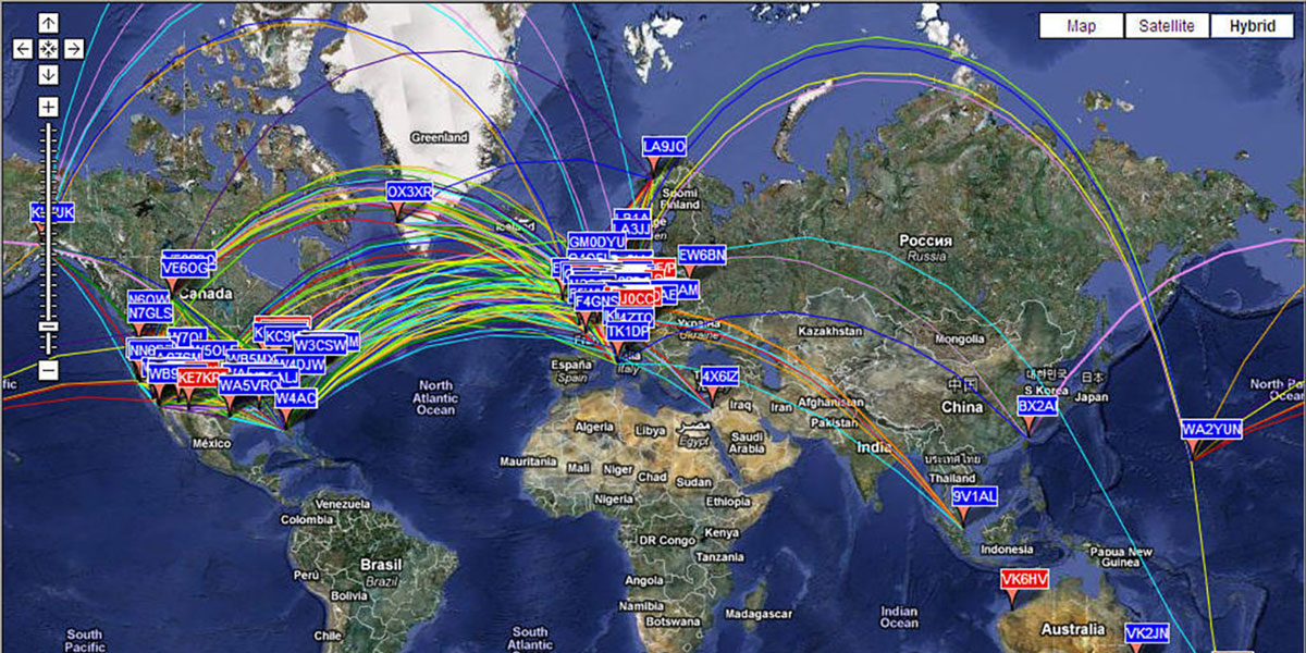
A particularly nice feature of WSPR is that “receptions” (called spots) can be automatically downloaded to a central database (wsprnet.org/drupal/) with results shown on a large map of the world (see Figure 1).
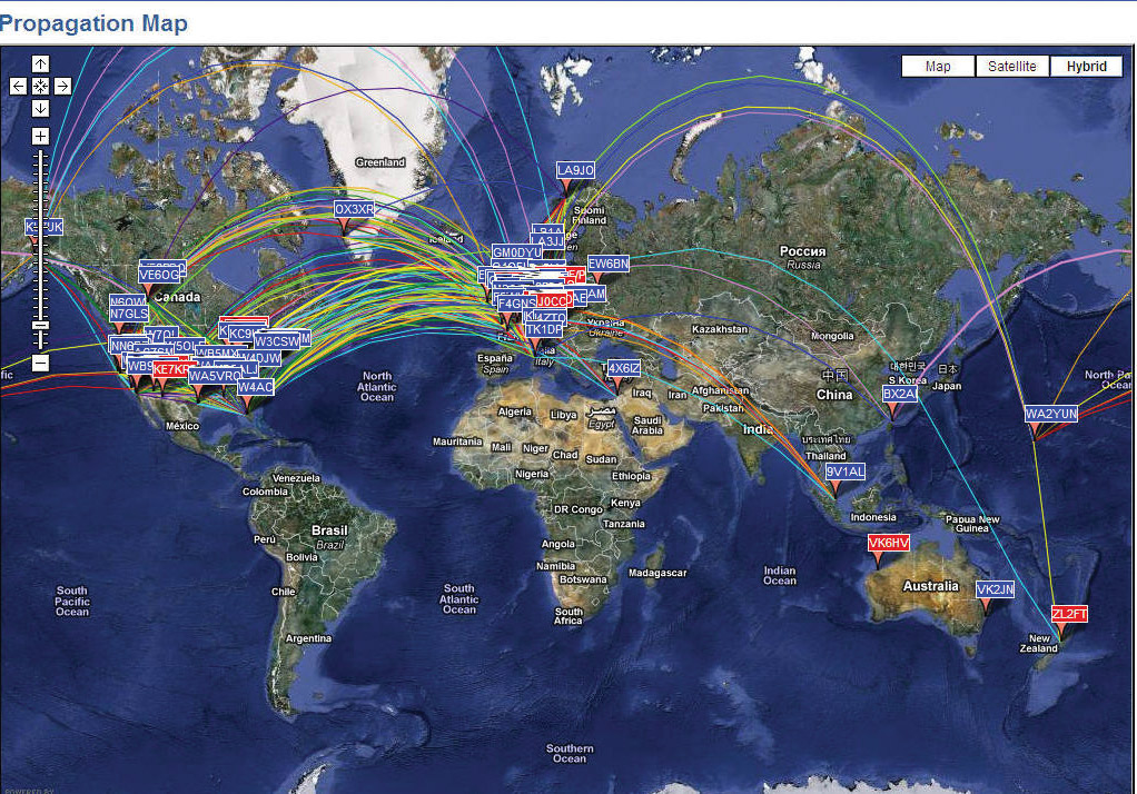
FIGURE 1. World map from WSPRnet.org/drupal/.
A flag will appear on the map to show your location and which stations you have received. Hence, exact transmitter locations can be determined and distances, headings, and other information reported. The world map can be zoomed to learn more about the geography and radio path found. Particularly thrilling for younger children is this reporting phase as they feel a sense of participation.
WSPR signals are in the amateur radio part of the spectrum and transmitters will require a license in most jurisdictions. Happily, many WSPR transmitters are now operating around the globe to provide interesting “catches” for the kids.
Why Do We Need WSPR?
We know from our high school physics class that when a transmitter signal moves down a wire to an antenna that part of it is launched into space as an electromagnetic (EM) wave. This energy propagates through space in various directions dependent on many factors, like the antenna size and orientation. All kinds of things can happen to the signal after it is launched. It can be refracted and polarized, for example. For communication, another antenna some distance away from the transmitter can intercept part of the signal and receive a message if one is contained in the signal. For example, Morse code is sent by turning the signal on and off (modulating it). Of course, for modern radio communications more advanced modulation methods are used. In an ideal universe, the EM wave would propagate forever and still be able to be demodulated perfectly at almost any distance with just the tiniest amount of signal available. However, in our real world there is another factor. In addition to the things mentioned above, we need to consider the ramifications of electrical noise.
As the EM wave propagates, it spreads out in space and therefore diminishes in strength in any given direction. Simply stated, it gets weaker. To add to the problem, the ionosphere — which carries much of the high frequency signals — also is continuously changing, causing propagation variations like fading. Noise, on the other hand, is all around our real universe being generated from all kinds of things like appliances, radar, and natural phenomenon like lightning. The noise level continuously fluctuates and causes interference to our signal.
To partially deal with the noise and also to provide additional features, various modulation techniques have been developed. Two classic ones you are probably familiar with are AM (amplitude modulation) and FM (frequency modulation). Some modulation methods are better than others at dealing with noise, but they all get into trouble when the signal strength approaches the noise level.
What makes WSPR different? It’s the protocol. WSPR software utilizes an extremely narrow frequency band with specially-coded forward error correcting (FEC) and frequency shift keying (FSK). FSK is like very narrow band FM. This technique reduces errors and improves the possibility of copying the message in noise. The signal fits into a tiny 200 Hz segment. Within each segment, the signal bandwidth is only 6 Hz. This allows several tens of stations to coexist in a segment with minimal interference. There are 12 segments presently (denoted here as the WSPR bands), located within the radio frequency spectrum (see Figure 2).
| Band |
Dial Freq. (MHz) |
Transmit Freq. (MHz) |
| 160m |
1.836600 |
1.838100 |
| 80m |
3.592600 |
3.594100 |
| 60m |
5.287200 |
5.288700 |
| 40m |
7.038600 |
7.040100 |
| 30m |
10.138700 |
10.140200 |
| 20m |
14.095600 |
14.097100 |
| 17m |
18.104600 |
18.106100 |
| 15m |
21.094600 |
21.096100 |
| 12m |
24.924600 |
24.926100 |
| 10m |
28.124600 |
28,126100 |
| 6m |
50.293000 |
50.294500 |
| 2m |
144.488500 |
144.490000 |
FIGURE 2. WSPR radio bands; center frequencies, bandwidth 200 Hz.
The WSPR protocol is extremely effective at signal-to-noise ratios as low as –28 dB in a 2,500 Hz bandwidth. This is over 10 dB below the threshold of audibility. In other words, you can sometimes copy signals that you cannot hear. It is because of this capability that even low power WSPR signals can be decoded in the farthest reaches of the globe.
WSPR Acknowledgement and Usage
WSPR was conceived and put into operation by Joe Taylor (K1JT), an amateur radio operator (Professor of Physics at Princeton) and fellow amateur Bruce Walker (W1BW). The open source software runs on Windows, Linux, and other systems. It is available from www.physics.princeton.edu/pulsar/K1JT as a free download.
WSPR utilizes the internal or external sound card of your PC/MAC (see Figure 3). These cards have good specifications.
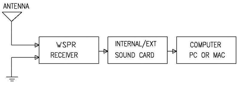
FIGURE 3. Typical sound card hookup.
Foremost are the data converters providing a large 90 dB dynamic range which is used to the fullest. WSPR is programmed to send and receive messages through the card. Here’s more about WSPR protocol.
WSPR uses time-synchronized communications based on Coordinated Universal Time (UTC). Transmissions last somewhat less than two minutes each, nominally starting one second into an even UTC minute. Hence, it is important for your computer to be accurate to within a second or so of UTC. So, set your computer clock to an accurate source such as the US Navy Master Clock.
Since most computer clocks drift, you will need to update your clock periodically.
WSPR is designed to do just one thing: find a communication path. It communicates via specially formatted messages aimed at determining if a propagation path is open on a given transmitting frequency. Formatting contains a name, four character grid locator, and power level in dBm (decibels relative to one milliwatt). This information is compressed into 50 binary digits and encoded using a convolutional code of length 32 and rate 1/2. The resulting 162 bits are transmitted using four tone FSK at 1.46 baud. The least significant bit is defined by a pseudo-random sequence known by the software at both transmitter and receiver. It is used to establish accurate time and frequency synchronization. Long convolutional codes are advantageous since undetected decoding errors are rare. Normally, a Viterbi algorithm is used for decoding but due to complexity, the WSPR decoder uses a special sequential algorithm.
When a station is decoded, other information such as “receive location,” name, S/N ratio, and DT (time difference) is routinely logged. This information can be automatically downloaded to WSPRnet.org/drupal/ using the “spots” option. Your name will then be shown on a flag on a world map with others. Options on the website can be used to find the distance and direction of the station received.
WSPR Receiver
What do we need to receive WSPR signals? First, realize that WSPR is transmitted as a single-side band (SSB) signal so it cannot be received with an ordinary AM receiver. Some shortwave radios have a BFO (beat frequency oscillator) and could be used if they possessed sufficient accuracy and stability. Also since the signal is in a very narrow band and almost inaudible, manual tuning would be difficult. Ham band receivers are another option, but more costly. So, it appears that finding a low cost WSPR receiver can be problematical. Is there another approach? Yes! Let’s design our own unique WSPR receiver from the ground up. On the hardware side, we need to build a WSPR receiver with high accuracy, stability, and sensitivity at low cost. In addition, it should not require complicated alignment or adjustment procedures involving special equipment. Quite a task.
Recall that the function of the receiver is to convert the WSPR radio signals to audio for the computer sound card. A good candidate for these requirements would be some type of fixed, direct conversion (DC) radio. DC receivers convert radio signals to audio directly without any intermediate stages. A block diagram of the proposed radio is shown in Figure 4. Here is how it works.

FIGURE 4. Block diagram for the WSPR receiver.
RF signals from the antenna are bandpass filtered at the WSPR receive frequency to prevent overloading the mixer from strong out-of-band signals. A local oscillator (LO) tuned to the WSPR transmit frequency is mixed with the RF. Since the two frequencies are separated by 1,500 Hz, audio centered at 1,500 Hz is produced at the output of the mixer. Finally, this audio is fed to the computer sound card. WSPR software has a 200 Hz bandpass centered on 1,500 Hz with narrow digital filters. So, if we get the audio to the sound card there is a good chance it will be decoded. Implementing the block diagram requires some unique thinking. First, we do not want an adjustable LO as this would require special equipment. Also, we do not want special coils that need to be tuned because measuring these would be difficult for many hobbyists. Figure 5 shows the circuit conceived. It functions like the block diagram.
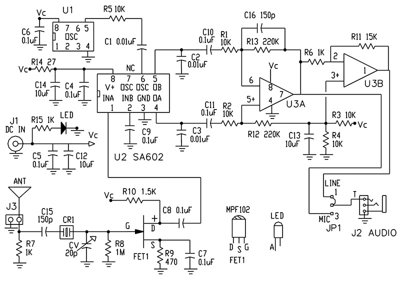
FIGURE 5. WSPR receiver schematic.
Two changes need more explanation. First, the LO is replaced with a programmed oscillator. This removes the need to adjust an oscillator. Programmable oscillators are essentially custom programmed crystal oscillators. Secondly, the input bandpass filter is now a crystal tuned to the WSPR frequency. Crystals provide a narrow band-pass function without using conventional tuned circuits. However, special crystal frequencies are required. Crystals for the 20 and 30 meter WSPR bands will be available as noted later. Here is a description of the circuit in Figure 5. From the antenna, the signal is passed through the crystal filter to a FET amplifier. Next, it is fed to one input (pin 1) of U2 — the SA612 mixer. The SA612 functions well in this application since it has gain (unlike passive mixers) and is protected from out-of-band signals by the crystal filter. Programmable oscillator U1 — programmed to a specific WSPR transmit frequency — feeds pin 6 of the mixer. The result is a differential audio signal on pins 4 and 5 of the mixer. This signal is further processed by U3 and presented to the sound card via JP1 and J2. Select the “line” or “microphone” jumper for your computer sound card.
The crystal filter may need peaking via the 20 pF variable capacitor CV. Since this is a sensitive place in the circuit, use care to avoid false readings. Adjust for maximum audio at 1,500 Hz. One way is to look at the audio spectrum with a free program like “Spectrum Lab,” from www.qsl.net/dl4yhf. A better method of alignment is to receive a nearby signal generator set to the WSPR receive frequency. Adjust CV for maximum while viewing the 1,500 Hz audio spectrum peak.
The circuit is powered by five volts through an AC to DC wall mount converter. Such converters can be troublesome. Check its voltage under load before using. Exceeding 5.5 volts may damage some parts. Using a computer USB port may work. We had good experience powering from the USB ports of some older laptops, but experience with other computers has produced strong interference from the USB port. In these cases, use the five volt wall mount converter.
For demonstration purposes, a breadboard of the 20 m receiver was built on a circuit strip shown in Figure 6.
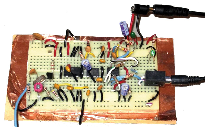
FIGURE 6. WSPR breadboard.
This technique, generally speaking, is not a good method for RF circuits but it worked here. A PCB is a better option.
Figure 7 gives the Parts List for the project. Most parts for the receiver are readily available. Programmable oscillators are available from Digi-Key and others as a custom order. You need to specify the package (usually eight-pin DIP) and frequency. Some special crystals are available on the Internet.
| QTY |
LABEL-VALUE |
DESIGNATION(S) |
DESCRIPTION |
| 8 |
0.1 µF |
C4, C5, C6, C7, C8, C9, C10, C11 |
Mono capacitor |
| 3 |
10 µF |
C12, C13, C14 |
Electrolytic |
| 2 |
150 pF |
C15, C16 |
Ceramic disc |
| 3 |
0.01 µF |
C1, C2, C3 |
Ceramic disc |
| 1 |
15K |
R11 |
1/4W 5% |
| 3 |
1K |
R15, R6, R7 |
1/4W 5% |
| 1 |
1.5K |
R10 |
1/4W 5% |
| 1 |
27 |
R14 |
1/4W 5% |
| 5 |
10K |
R1, R2, R3, R4, R5 |
1/4W 5% |
| 1 |
470 |
R9 |
1/4W 5% |
| 1 |
1M |
R8 |
1/4W 5% |
| 2 |
220K |
R12, R13 |
1/4W 5% |
| 1 |
3SIP |
JP1 |
SIP3 |
| 1 |
MPF102 |
FET1 |
FET |
| 1 |
LED |
GREEN |
LED |
| 1 |
20p |
CV |
VAR C |
| 1 |
J1 |
DC |
JACK 3.5 mm |
| 1 |
J2 |
AUDIO |
3.5 mm stereo |
| 1 |
J3 |
ANT |
Two terminal |
| 1 |
U2 |
SA612 |
RF mixer |
| 1 |
U3 |
TLC272 |
Dual op-amp |
| 1 |
U1 |
Programmable OSC |
WSPR transmit freq |
| 1 |
CR1 |
Crystal |
WSPR receive freq |
FIGURE 7. Receiver Parts List.
WSPR Software and Receiver Operation
Using the WSPR software is easy. To get started, download and run the software from www.physics.princeton.edu/pulsar/K1JT. Two windows will appear on your screen. The black one is for error messages. Figure 8 shows the main window. To check operation, you can play back an audio sample included with the program. If you want to check out actual band activity, use WSPRnet.org/drupal/ for current spots.
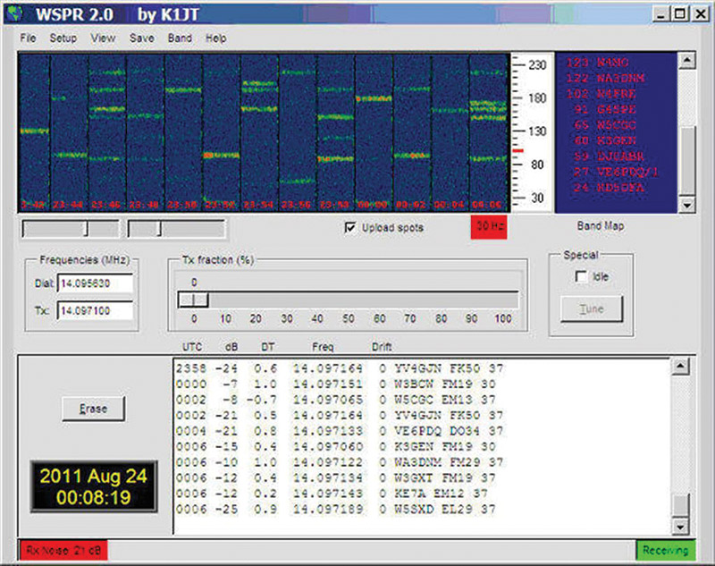
FIGURE 8. WSPR operating window.
Assuming you have a receiver, connect it to a good antenna and the audio output to your sound card. A long antenna high in the air working against a good ground works best, but even a random length wire works. If possible, try to make your antenna one-quarter wave long as it will better match the input. For example, on the 30 meter band make the wire 7.5 meters long (24.6 feet). It cannot be over stressed that a good ground helps enormously. Even a long ground wire on the floor helps. Keep the antenna away from the computer. Using a short coax cable may help.
Now, set your computer clock to UTC within one second or so. Correct UTC can be found on the Web. We use the Naval clock. Now comes the anxious part. You need to wait for an even numbered minute (0, 2, 4, etc.) for the software to begin receiving. Watch your computer clock. At this point, the message in the lower right corner will change from “waiting” to “receiving.” The lower left corner will specify the level of the input audio in dB. This can be adjusted with your sound card recording level control.
A level of 12 to 19 dB works well, even though the software says otherwise and produces a red window. There are a few other things you can do, like putting in your grid location and call (or name) if you want to report your spots. But that will come later. For now, sit back and watch for your first catch.
Final Comments
WSPR is amazing technology. The simplicity of the WSPR receiver described here makes it attractive as a low cost radio propagation tool. With a bit of luck, it will motivate experimenters, teachers, and students to begin exploring the many facets of science and engineering touched upon here.
As stated, the question, “How does that work?” is indeed the key to curiosity. Hopefully, it will help the young stay interested in science.
This receiver is only the first step. Other projects involving more sophisticated receivers and transmitters will surely follow. There was an article “Chips In Space” by Mason Peck (IEEE Spectrum August ‘11) which described how satellites the size of small integrated circuits could revolutionize the way we explore space. Project Sprite involves designing and later on launching many thousands of low mass chips (under 50 milligrams) for the single purpose of monitoring space with simple sensors. Each chip will have a weak radio transmitter and signal barely discernable from noise. Sophisticated signal processing software will be needed to pull the signals out of the noise.
Perhaps a youngster intrigued by WSPR will be the future engineer to design that software. NV