Want to hear the world turning? You can — it’s right behind the front panel of a radio!
In Part 1, we covered a batch of basics: definitions of terms, and some fundamentals of how waves travel about. Not only hams can take advantage of radio propagation — everybody has a chance to experience some very interesting ways of interacting with the natural world through wireless. Let’s put that know-how to work!
The Radio Horizon
To most people, “using a radio” means the short-range “walkie-talkies” used by public safety agencies and as the Family Radio Service “walkabouts” available to everyone. If pressed, they might also realize that mobile phones, Wi-Fi, and even Bluetooth links are a type of radio, too. The expectation for all those radios is the signals can only be heard within “line-of-sight” range.
A radio wave traveling between two points within line-of-sight range of each other — without bouncing off or bending around anything — is called the space wave. How far can a space wave travel between two stations? On a really, really clear day in a wide open area like the Great Plains, you can actually see all the way to where the curvature of the Earth blocks your view of anything more distant. This is the geometric or optical horizon. The farther you are above the ground, h, the farther you can see, d, according to the formulas:

Typically, humidity and dust obscure the view and you can’t really see that far. At the longer wavelengths of radio, the distribution of impurities in the air cause radio waves to travel very slightly faster at higher altitudes. As the speed of the wave changes, the wave is refracted or bent very slightly, just like when light is refracted when it changes from one medium to another. (Think of the classic demonstration with a pencil in a glass of water appearing to bend at the water’s surface.) This refraction — while slight — causes the radio waves to gradually bend back toward the Earth’s surface so they can be “seen” at longer distances than light. This is the radio horizon.
The distance to the radio horizon also depends on height, as shown in Figures 1A and 1B. Figure 1A shows a transmitter (T) and a receiver (R) with antennas located at heights H and H1, and radio horizons D and D1, respectively.
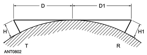
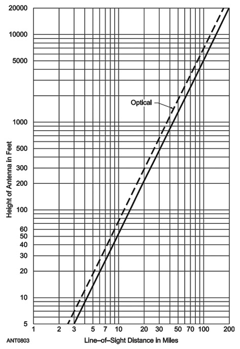
FIGURE 1. Line-of-sight distance between two stations is determined by the height of each station (A). The chart at B shows the distance of both the optical and radio horizons for a single station. Determine the horizon distance for each station and add them for the total line-of-sight distance between the two stations. Graphic courtesy of the American Radio Relay League.
The chart (Figure 1B) shows how to determine D and D1. Just find the radio horizon distance for each station and add for the longest possible radio line-of-sight distance. (Note the dashed line in Figure 1B showing the slightly shorter distance to the optical horizon at equal heights. In the previous equations, change the constants to 3.86 and 1.32 to calculate the radio horizon.)
Ground Wave
This atmospheric refraction becomes less effective at lower frequencies (longer wavelengths). Below VHF (see the sidebar on Frequency Range Abbreviations) in the HF and MF range, the space wave is still important but another phenomenon becomes significant: ground-wave propagation.
Radio waves can travel along any surface or interface between two media in which the wave travels with different velocities. The surface of the Earth is a good example and waves do travel along it. Known by its technical name of “dirt,” the Earth is actually quite lossy at almost all frequencies, converting the electromagnetic energy to heat, or “worm burning” as hams call it. So, as the wave travels along the ground, it is rapidly attenuated.
Ground loss gets higher with frequency, so the ground wave is most effective at and below HF. The typical range of a 10 meter (28 MHz) or CB (27 MHz) ground wave signal is about 5-10 miles depending on the terrain. At AM broadcast frequencies in the MF range (0.5 to 1.8 MHz), the ground wave can be received out to 100 miles or so. That’s why you can listen to the local AM stations even well past the calculated radio horizon.
Frequency Range Abbreviations
| MF (Medium Frequency) |
0.3 to 3 MHz |
| HF (High Frequency) |
3 to 30 MHz |
| VHF (Very High Frequency) |
30 to 300 MHz |
| UHF (Ultra High Frequency) |
300 to 3,000 MHz |
| SHF (Super High Frequency) |
3 to 30 GHz |
| EHF (Extremely High Frequency) |
30 to 300 GHz |
Tropospheric or Weather-Related Propagation
Remember that statement about changes in wave velocity causing the wave to bend? In Part 1, you learned that wave velocity is determined by the permittivity and permeability of whatever medium the wave travels through. Permittivity is what determines a material’s dielectric constant — the same dielectric constant used to determine capacitance.
So, wherever dielectric constant changes, the wave’s velocity and thus its direction also change. Does this happen in the atmosphere? You bet!
There are a lot of instances in which the dielectric constant changes — often abruptly — in the lower atmosphere, known as the troposphere. These are caused by weather-related events: storms, cold and warm fronts, even temperature inversion layers.
Anywhere there is an abrupt change in the atmosphere, the effect on radio waves is almost as if they were reflected from the air having a different dielectric constant. Propagation of radio waves between two points by using this reflecting effect (even though it’s really a sharp bend created by refraction) is called tropospheric propagation or just “tropo” by hams.
Figure 2 shows a typical example of how tropo might occur along the inversion layer that builds up whenever there are stable conditions near the ground. A layer of warm air — often humid and dusty — builds up but is trapped under the cold dry air above.
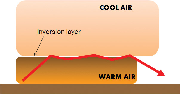
FIGURE 2. The inversion layer between warm air trapped near the ground and colder air above it. The change in dielectric constant between the two regions causes refraction of radio waves and can conduct the waves along the inversion layer for long distances.
You can see where the inversion layer is from a plane when taking off or landing — it’s the darker colored air on which the clouds seem to rest. If you can launch a radio signal along this layer at a shallow angle, it can travel for quite a distance! Tropo contacts from this and similar effects can be made at VHF and UHF frequencies — even microwaves — over hundreds of miles.
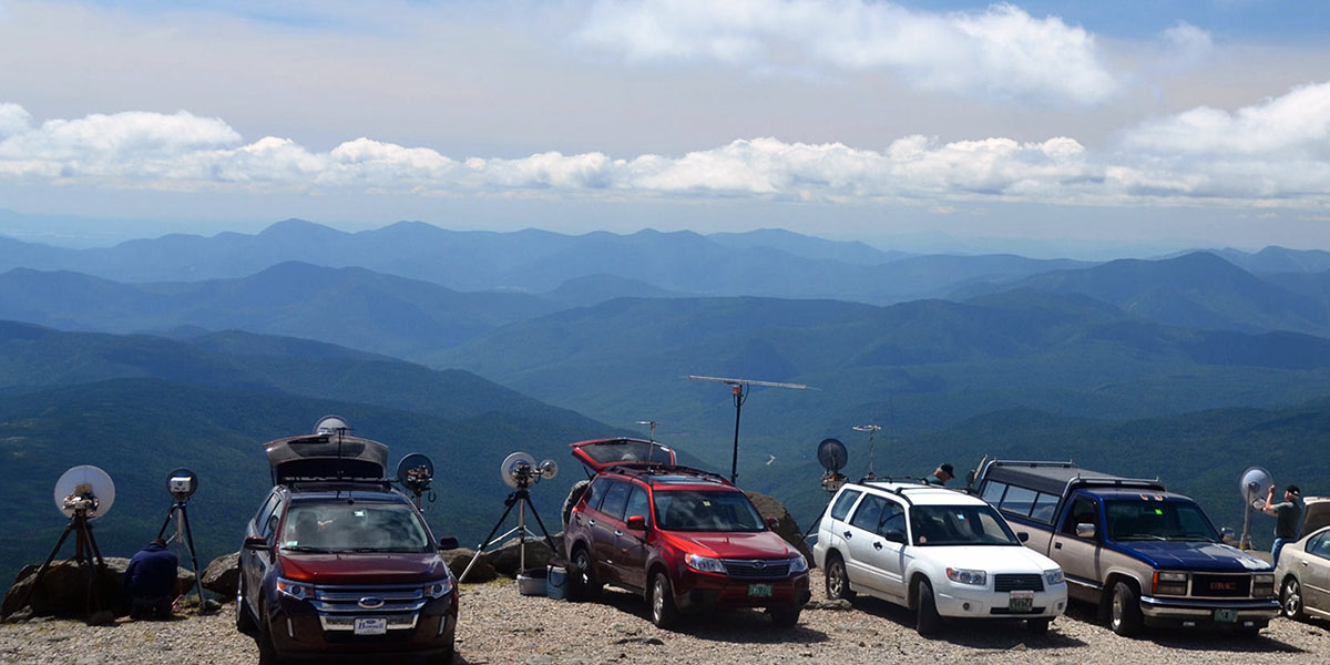
During microwave contests, hams put up portable stations at high places (such as in Figure 4), hoping for the best possible angle for tropo.
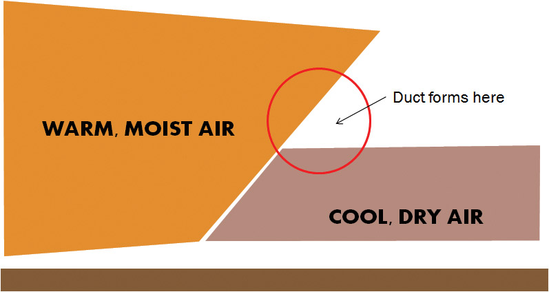
FIGURE 3. A duct can form between two layers of air with different properties or (as shown here) along a weather front. In this case, the warm moist air of a storm system has pushed over the top of a cooler layer, creating two separate refracting "walls." Signals can be trapped in the duct until one of the layers disperses, allowing signals to reach the ground again.
Since you can’t “see” tropo, how do you know when it’s happening? A surprisingly easy way is available to everyone by using an ordinary FM broadcast receiver and a simple outdoor antenna, such as a folded dipole or combination TV-FM antenna. Tune your receiver to an unused channel and set the receiver to “Mono” which usually enables audio output even if no signal is present.
If you can aim your antenna, point it at a city or region 300 miles or so away with an FM station on that channel — well past the radio horizon. Then, listen on a day when the atmosphere is quiet and stable.
If tropo occurs, you might hear the station fade in (perhaps surprisingly strong) for a few minutes or longer. You’ve just become a tropo DXer! (“DX” stands for distance.)
But Why A Duct?
One variation of tropospheric propagation is referred to as “ducting.” This occurs when more than one reflecting (remember, it’s really refraction) layer is present. A signal can be trapped between the layers and bounce between them until one layer disappears and lets the signal out of the duct.
Figure 3 gives a typical example of how ducts are created by a storm front. Whenever a strong front moves through your area, that’s a good time to have your FM receiver on and listening to that “empty” channel. You may get a big surprise!
Hams know to aim their antennas parallel to the front as it moves through, hoping for a duct to form and carry their signals far from home.
Another way to predict when tropo might happen is to use Hepburn maps. Created by William Hepburn from weather data, these maps (www.dxinfocentre.com/tropo.html) show when and where atmospheric conditions are right for tropo. You can also keep an eye on the real time ham radio contact maps at www.dxmaps.com/spots/map.php to see if any activity is being reported.
Spring and summer are the best seasons for tropo, although it can occur anytime there is favorable weather.
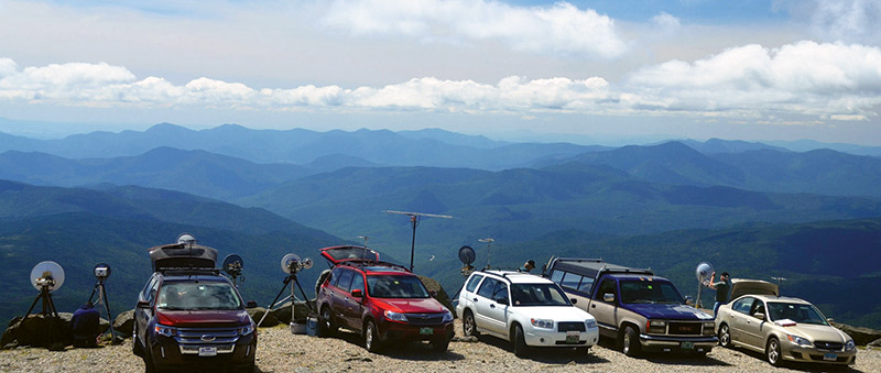
FIGURE 4. Using portable dish antennas, these hams are attempting to launch 10 GHz signals along the inversion layer that can be clearly seen at the bottom of clouds over the Mt. Washington, NH region.
Does Propagation Really Matter?
To most short-range links like Bluetooth and Wi-Fi, line-of-sight and tropo don’t have a significant effect. Once you start considering longer range point-to-point links or receivers on the tops of buildings or hills, you should be aware of the potential for tropo to disrupt communication. Hams may enjoy “working DX” over long distances but it you’re just trying to shovel bits, a signal from far away is not something you want to receive.
Interfering signals or distortion caused by multi-path from ducts or inversion layer propagation can shut down a comm link or cause loss of contact with a mobile or airborne platform.
Be aware of the possibilities and have a “plan B” in mind — either on a different frequency band or by aiming your antenna in a different direction.
Shortwave Propagation
The “real DX” comes from propagation using an entirely different — and much higher — region of the atmosphere. Starting at about 30 miles above the ground, the ionosphere can bend radio signals back towards the ground where they are received thousands of miles away. The ionosphere is almost a vacuum; in fact, the International Space Station is actually orbiting in the very top of the ionosphere — so how can it refract a radio wave?
The key is in the name. “Ion” refers to the effect of solar ultra-violet (UV) radiation on the sparse collection of gas molecules in the upper atmosphere. The UV is ionizing radiation energetic enough to free an electron from an atom, creating two free electrically-charged particles: a negative electron and a positive atom. If enough atoms are ionized in this way, both the permittivity and permeability of the ionosphere change enough that it can refract a radio wave. If the wave is bent enough to return to Earth, that is sky-wave or “skip” propagation.
Ionization is created and disappears each day as the Sun illuminates different parts of the Earth, forming into several distinct layers or regions: D, E, and F as shown in Figure 5.
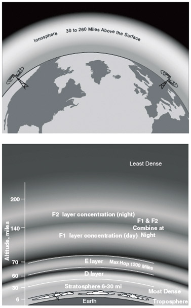
FIGURE 5. The ionosphere forms daily at heights of 30 to 260 miles. Due to variations in density, several different layers are formed, each having a different effect on radio waves. Graphic courtesy of the American Radio Relay League.
(The F layer can further split into the F1 and F2 layers during hours of peak illumination.) The D layer is the lowest at around 30-50 miles, with the E layer just above it; the F layers are found at 60-260 miles.
Each layer has different properties and creates different effects as experienced on the ground. (There are also seasonal effects due to the tilt of the Earth’s axis.)
The lowest layer (D) acts mostly as an absorber of radio energy. It is the D layer that soaks up AM broadcast signals during daylight and limits reception to ground wave range. Immediately after sunset, the free electrons recombine with the ionized atoms and the D layer disappears.
AM signals can then be bent back to Earth by higher layers and long distance sky-wave reception becomes possible after sunset.
There is a thriving community of “broadcast DXers” who specialize in picking up distant AM stations — sometimes even across oceans.
The E layer — next highest in the stack — is a bit of a mysterious place. Too high to be dense enough for absorbing RF and too low to create reliable long distance communication, its main claim to fame is for reflecting regions called sporadic E or Es clouds. These patchy regions of ionization are thought to be created by wind shear, compressing metallic ions and dust particles into thin layers.
When ionized by solar UV, these thin layers reflect signals back to Earth, enabling contacts to be made over an average of 1,200 miles. While your FM receiver is on, you may hear stations appear very quickly with good signal levels, last for a while, then fade just as quickly — that’s probably due to Es.
Hams operating at 50 MHz enjoy “E skip,” dubbing those frequencies the “Magic Band” for the highly variable — but exciting — propagation far beyond the usual range.
Finally, the F layers are where the real long distance action is for frequencies below 30 MHz — the traditional shortwave bands. In the highly rarified upper reaches of the atmosphere, gas density is very low and the ionized regions may last all day before recombining at night.
Low density also means it takes a lot of UV to return a signal to Earth — especially at the higher frequencies where less bending occurs. In fact, if the frequency is too high, the signal is eventually lost to outer space as shown in Figure 6.
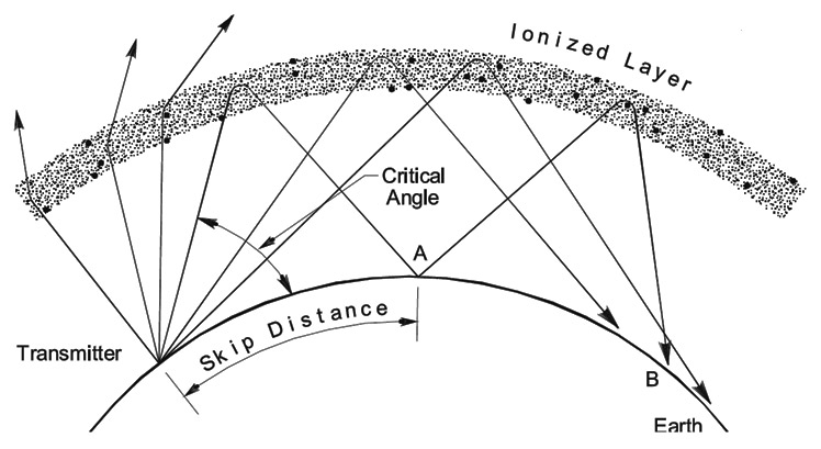
FIGURE 6. The ability of the ionosphere to return signals to Earth depends on the signal frequency and the vertical angle at which the signal encounters the ionosphere. At a sufficiently high vertical angle, the signal cannot be bent enough and is lost to space. The critical angle at a given frequency is the highest vertical angle at which a radio signal of that frequency can be returned to Earth. Graphic courtesy of the American Radio Relay League.
Solar Effects
With the ionosphere so dependent on solar UV to exist, it is strongly affected by events on the Sun. The most significant long-term relationship is driven by the 11 year (10.7 years, actually) sunspot cycle in which the number of spots waxes and wanes. More spots equals more solar flux equals better HF propagation equals happy hams and shortwave broadcast listeners!
In the short-term, the Sun is a highly variable source of propagation excitement. Solar flares and coronal mass ejections occur nearly every day at scales from nearly indetectable to massive. Coronal holes and the solar wind send charged particles streaming away from the Sun.
When they encounter the Earth's geomagnetic field, the fun really begins, creating the auroras and other interesting phenomena that can enhance, disrupt, or even shut down HF propagation entirely.
Numerous websites are dedicated to watching the Sun and its effects here on (or rather, above) the Earth.
Assuming the signal is returned to Earth, the distance at which it reaches the ground again is called the skip distance, and one such up-and-back trip is called a hop. Typical hops involving the F layer span from 1,500 to 2,500 miles on the higher HF ham bands from 14 to 28 MHz.
Note that the signal can also be reflected by ground or water, then make another hop. That’s how contacts span the thousands of miles between North America and other continents.
Even though each hop attenuates the signal by about 20 dB (a factor of 100), modern antennas and transceivers are good enough for “solid copy” — even between stations at opposite sides of the planet when conditions are right.
Predicting Propagation
With all this activity and inter-related effects, is it possible to predict ionospheric propagation as Hepburn maps do for tropo? Yes, and the models are surprisingly accurate! A lot of time and effort was expended studying and modeling HF propagation, resulting in a number of software packages that are used by various communication services, including hams. In fact, one of the best was developed in support of Voice of America broadcasts. It’s called VOACAP Online and you can experiment with it yourself for free at www.voacap.com.
There are two basic but very useful ways to use the program: coverage mode (Figure 7) and prediction mode (Figure 8).
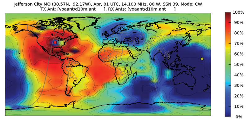
FIGURE 7. VOACAP Online coverage map from Jefferson City, MO at 8 PM in April on the 14 MHz amateur band for stations using half-wave dipole antennas at a height of 10 meters and CW (Morse code). Coverage should be excellent across the Americas, west Africa, and much of the eastern Pacific with current sunspot activity values.
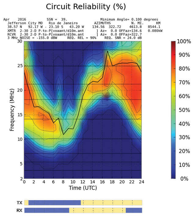
FIGURE 8. VOACAP Online prediction chart for circuit reliability between Jefferson City, MO and Rio de Janeiro with the same stations and solar activity as in Figure 7. The heavy black line represents the MUF — Maximum Usable Frequency — at which communications are possible 90 percent of the time.
Coverage mode answers the question, “Given certain station capabilities, where can I expect to make contact on a specific frequency at a given time and date?” Prediction mode answers a more specific question, “On what frequencies and at what times can my station make contact with a specific area on a certain date?”
Give it a try. In coverage mode, select your location from the menu, specify a simple wire dipole antenna at 30 feet for both receiving and transmitting stations, pick one of the shortwave bands, and click “Run the Prediction!” You’ll get a colorful map like Figure 7 showing you where that basic station could make contacts at the time you run the program.
Change the date or time — you’ll be surprised at the extent of the changes. You can change from Morse (CW) to one of the voice modes (AM or SSB), change the type and height of the antenna, or see what happens on different bands.
Maybe you have a cousin in Timbuktu. Enter the prediction mode, set up your station, frequency, and time and date to find out when you could have an on-the-air chat. It’s really a fascinating program. Not as fascinating as getting a ham license and actually doing it, but fun and educational nevertheless.
References
Of course, we’ve only scratched the surface of what radio propagation is all about. We started with the basics and now you can see a few of the interesting opportunities for experimentation. The references listed in the sidebar will help you learn a whole lot more.
Maybe we’ll even hear you on the air giving propagation a workout! NV
References
ARRL Antenna Book
An extensive collection of antenna designs with a detailed chapter on propagation from MF through microwaves.
https://www.arrl.org/shop/ARRL-Antenna-Book-Softcover/.
ARRL RF Propagation
Links to articles and resources dealing with propagation.
www.arrl.org/propagation-of-rf-signals.
Don’t forget the ARRL Tech Portal.
www.arrl.org/tech-portal.
Spaceweather
Daily news and articles about phenomena in space, on the Sun, and here on Earth.
www.spaceweather.com.
Spaceweather Prediction Center
Real time information on shortwave propagation conditions, including solar and geomagnetic activity.
www.swpc.noaa.gov/communities/radio-communications.