Much as we learn about ourselves from our mistakes, we can learn a great deal about transformers from their imperfections. Most electronics hobbyists understand the basic principles of ideal transformers; that the winding voltages are directly proportional to turns, currents are inversely proportional to turns, and an impedance connected to one winding is seen from the other winding as being multiplied by the square of the turns ratio. Figure 1 illustrates these fundamentals.
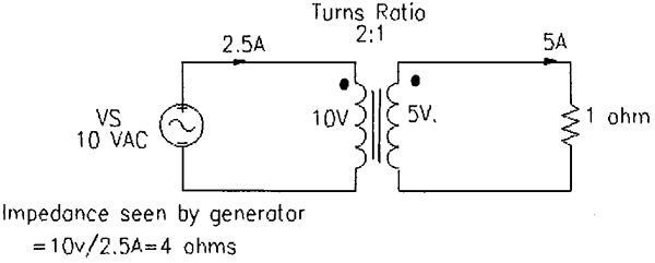
FIGURE 1. Ideal Transformer Principles Illustrated
However, all these conditions are only applicable if:
- All of the magnetic field generated in the any one winding links and induces voltage in other windings
- There is negligible resistance in either or all of the windings
- There is no hysteresis or eddy current loss in the core
- The self-inductance of the excited winding approaches infinity, so that the magnetizing current that produces the flux in the core is near zero
- Capacitance effects are negligible
While many iron core transformers operating at low frequency come remarkably close to meeting some of these criteria, none actually completely meet any of them, and hence never quite live up to the ideal principles stated above. For some purposes it is okay to assume ideal transformers, but for others it is necessary to consider the imperfections of the devices.
The equivalent circuit of Figure 2 is helpful in visualizing the transformer’s imperfections. In this two winding transformer, Rs represents the combined AC winding resistances of the primary and secondary windings. The term Xs represents the winding “leakage reactance.”
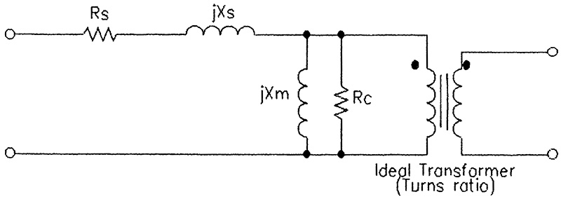
FIGURE 2. Equivalent Circuit with Lumped Winding Resistance and Leakage Reactance
In an ideal transformer where every line of magnetic flux generated in the primary winding links the secondary windings and vice versa, flux generated by the load currents would completely cancel in accordance with Lenz’s Law, and the core flux would remain constant for all load conditions.
In a real transformer, however, flux linkage is not perfect, and the transformer introduces inductive reactance, usually small, in series with the circuit.
The parallel resistance Rc represents the energy losses due to hysteresis and eddy currents in the core. These are real energy losses and hence can be represented by resistance. The parallel reactance, Xm, is the inductive reactance of the excited winding, and it is the current in this branch that produces the principal magnetic field in the core. The turns ratio is represented by the ideal transformer, the dots showing terminals which have the same instantaneous polarity.
Values for the resistance and reactance components in the equivalent circuit are readily obtained from two simple tests: an open circuit or no load test in which one winding of the transformer is energized at rated voltage with the other winding(s) open; and a short circuit test in which voltage on one winding is applied to achieve rated current with the other winding(s) short-circuited.
In both tests, voltage, current, and power are measured on the energized winding. See Figure 3.
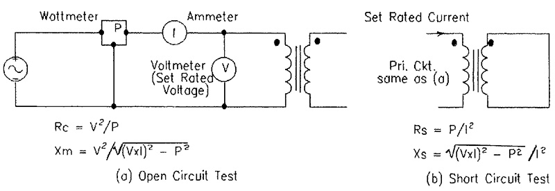
FIGURE 3. Instrumentation for Tests and Formulas for Calculation of Equivalent Circuit Parameters
The current in the open circuit test will be quite small, so that the power losses and voltage drops in Rs and Xs are considered negligible, and it is assumed that all power losses are core losses (hysteresis plus eddy current). The core parameters Rc and Xm are calculated as shown in Figure 3a, using applied voltage. The series parameters — Rs and Xs — are calculated in a similar manner from the short circuit test.
In this test, the voltage will be much less than rated voltage, and it is assumed that core losses, which are voltage sensitive, are negligible. While the instrumentation is basically the same as for the open circuit test, it is now the current through the series elements which is known, rather than the voltage across the the parallel core elements. See Figure 3b.
While the above tests are normally associated with large power transformers, the same principles should apply reasonably well to small transformers with some loss of accuracy. To make the point, an off-the-shelf transformer rated 120 to 12.6 volts, 1.2 amp, was purchased at a local electronics store and tested with the results shown in Table 1.
| |
V1 (volts) |
I (amps) |
P (watts) |
V2 (volts) |
| Open Circuit Test |
120 |
0.048 |
2.30 |
14.4 |
| Short Circuit Test |
13.83 |
0.126 |
1.63 |
0 |
TABLE 1 — Test Data on Transformer Rated 120V to 12.6V @ 1.2A, 60Hz
Using the methods described previously, the equivalent circuit shown in Figure 4 was developed.
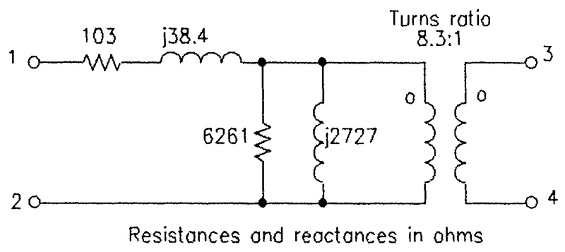
FIGURE 4. Equivalent Circuit of Tested Transformer
Impedance transformation is not only an important application of transformers, but enables us to further simplify the equivalent circuit. To understand how impedance transformation works, refer back to Figure 1. By tracing back from the load resistor to the source generator using ideal transformer concepts, it is easy to see that the generator sees an impedance which is a2 times the load impedance, where a is the turns ratio, N1/N2.
If we interchanged the source and load, the impedance seen by the source would be divided by a2, again with a = N1/N2, to give an apparent resistance of one ohm. One very common application of this principle is in matching the impedance of an amplifier to that of a speaker so as to optimize power transfer in accordance with the maximum power transformer theorem.
We may also use this principle to eliminate the ideal transformer in the transformer equivalent circuit and thus provide for analysis at a single voltage level.
Consider the 120 to 12.6 volt transformer described previously connected to a 120 volt, 60 Hz source and with a resistance load of 10 ohms connected to the 12.6 volt winding.
The complete equivalent circuit, neglecting source impedance, is shown in Figure 5a. The same equivalent circuit with the load resistance referred to the source side is shown in Figure 5b. This was accomplished by simply multiplying the 10-ohm load by (8.3)2.
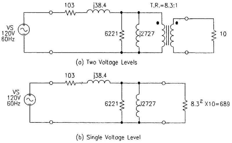
FIGURE 5. Equivalent Circuits with 10 Ohm Load
In many instances, it is more convenient to work from the low-voltage side of the transformer rather than the high-voltage side.
The same principle used to refer the load impedance to the source side in Figure 5 can be used to refer all impedances to the low-voltage side.
To accomplish this, we divide all high side impedances by a2. Again, in the example used above, we convert the transformer equivalent circuit to the 12.6 volt side by dividing high side impedances by (8.3)2 and placing the ideal transformer at the high voltage terminals. See Figure 6. (This is the same transformer equivalent circuit that would be obtained if the unit was tested from the low-voltage side.)
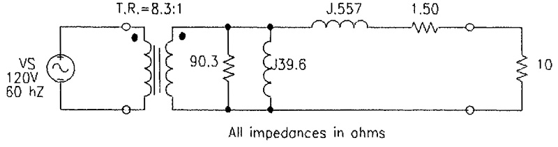
FIGURE 6. Equivalent Circuit Referred to Low Voltage Side
Circuit analysis using a complete equivalent circuit as described above can be fairly tedious, and requires skill at complex algebra techniques. Fortunately, for many purposes, including most small transformer applications, substantial simplifications are possible.
While the parallel magnetizing branch components — Rc and Xm — introduce some error in the ideal current transformation ratio, their effects on circuit behavior are often minimal in comparison with the series components — Rs and Xs — and consequently may often be omitted.
This results in a very simple equivalent circuit, consisting of merely a series impedance and an ideal transformer, or, if all parts of the system are referred to a single voltage level as in the preceding paragraphs, of just a series impedance.
Moreover, in small transformers such as that described in this article, the series resistance — Rs — is usually much higher than the leakage reactance, Xs, so that Rs + jXs does not differ greatly from Rs. Thus, Xs for small transformers can often be neglected, which allows us to reduce the equivalent circuit to a mere series resistance.
To illustrate, suppose we wish to find the secondary voltage of the transformer described previously when the load on the full secondary winding is 25 ohms. If we reflect this resistance to the primary side so as to eliminate the turns ratio, we have 8.32x25 = 1722 ohms. Our ultra-simplified equivalent circuit is then as shown in Figure 7.
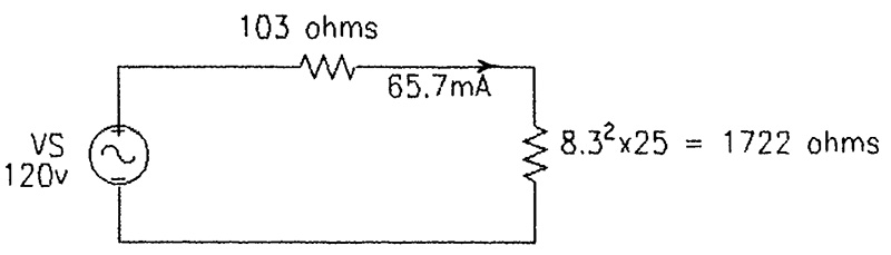
FIGURE 7. Ultra Simplified Equivalent Circuit with 25 Ohm Load
With 120 volts applied, the primary current is 120/(103+1722) = 66 mA, and the drop across the load — referred to the primary — is .066x1722 = 114 volts. Now, we re-insert the turns ratio, and our secondary voltage is 114/8.3, or 13.7 volts.
We can check the legitimacy of our approximate equivalent circuit by calculating the secondary voltage at full rated load; it should be 12.6 volts.
The full load resistance is 12.6/1.2 = 10.5 ohms, which is 8.32x10.5 = 723 ohms reflected to the primary. The resistance seen from the source is 723+103 = 826 ohms, and the primary current is 120/826 = 0.145 amperes.
The load drop referred to the primary is 0.145x723 = 105 volts.
Finally, dividing 105 volts by the turns ratio of 8.3 gives us 12.65 volts, which is very close to the winding rating of 12.6 volts.
A solution using the complete equivalent circuit and complex algebra yielded a load voltage of 12.638 volts. NV