A voltmeter, signal generator, and a few parts combine to make a powerful impedance measuring tool.
Measuring the impedance of an antenna, a component, or a circuit such as a matching network, can often help us optimize our equipment and improve our understanding of its operation.
Commercial network analyzers, RF impedance meters, or antenna analyzers can do the job, but are out of the realm for many amateurs, especially since the equipment is expensive and would be sitting idly on the shelf most of the time. If we only need a few measurements, an old technique — the three voltmeter method — that uses a signal generator (or a QRP rig) and the ubiquitous digital voltmeter may fill the bill.
These items together with a few dollars worth of parts, a bit of software, and some manual work on your part can produce the data you need in just a few minutes. It also provides an easy, low cost way of acquainting yourself with the art of impedance measuring. While not as convenient as some commercial equipment, there is a satisfaction that comes with building and understanding a device that you have built yourself.
Discussed in this article are the details of this unusual RF impedance analyzer which uses a simple circuit with diode RF voltage samplers, as well as software for your PC that processes the data, compensates for the diode nonlinearities, and calculates the impedance, SWR, and other parameters of interest at frequencies up to 21 MHz or more.
This approach to impedance measurement has its limitations, but on the plus side, it is an easy project to build, is low cost, requires no power supply, and has the capability of producing results comparable to equipment costing much more.
If you decide to build the project, you will need a PC running Windows®, a signal generator to cover the frequencies of interest with at least 13 dBm output into 50 ohms (about 1.414 peak volts or 20 mW), and a high input impedance digital voltmeter (DVM) with a DC accuracy of at least 0.5%. The circuitry is very low cost (less than $5) and uses readily available parts. I suggest that you build the circuit inside of a metal enclosure (not a solderless breadboard like I did) since that would limit your frequency range. To get started, let’s review some concepts of impedance.
Impedance Models
Impedance is the more complete expression defining current flow than resistance alone and is typically expressed as a complex quantity such as R + jX where R is the resistive part (real) and X is the reactive part (imaginary). The reactive part is usually frequency dependent and is preceded by the math operator “j” to indicate it is the imaginary part. For many resistors, the reactive part is very small, except for wire wound types. And so, it is typically ignored.
On the other hand, many inductors and capacitors are lossy (as seen in Figure 1) and have both a resistive and reactive part with the reactive part being positive for inductors and negative for capacitors. Measurements made on transmission lines and antennas also show both a resistive and reactive part which can be either inductive or capacitive, depending on the measuring frequency.
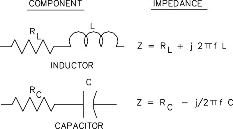
FIGURE 1. Lossy series models of inductor and capacitor. Frequency f, in hertz, resistance R, in ohms, inductance L, in henrys, and capacitance C, in farads.
The models of Figure 1 show the resistive part modeled in series with the reactance. Another model is sometimes used with parallel resistors as shown in Figure 2. The series and the parallel models are equivalent at the same frequency of measurement and can be converted from one to the other using the equations shown on Figure 2.
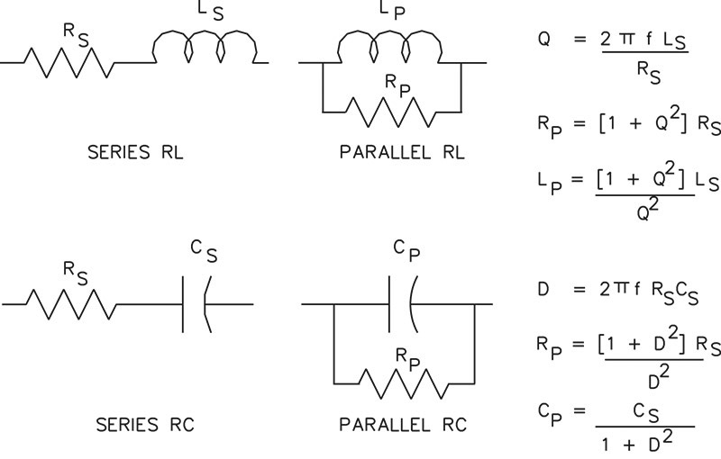
FIGURE 2. Series and parallel equivalent circuit models at the same measuring frequency.
The impedance analyzer software (discussed later) basically calculates the impedance in polar form from voltage measurements provided to it. This can be converted to rectangular form as shown in Equation 1:
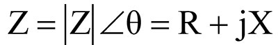
EQUATION 1.
where Z is impedance in ohms, |Z| is the magnitude of Z, θ is the angle of Z, R is the resistive part of Z, and X is the reactive part of Z. The two forms in Equation 1 are related by:
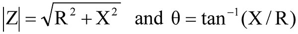
EQUATION 2.
The impedance analyzer program will display the results in both polar and rectangular form on the computer screen. From here, it is relatively easy (knowing the measurement frequency) to calculate the values of the series and parallel models and to display them on the screen. Other parameters such as the Q (quality factor), or D (dissipation factor), SWR, and reflection coefficient are also calculated and displayed. Now let’s see how to measure impedance in polar form using just a voltmeter.
Three Voltmeter Method
In previous articles [1, 2], I described a powerful method of measuring impedance at audio frequencies using a simple circuit and a computer with a sound card. Briefly mentioned was the “three voltmeter method” (TVM) as one technique that was looked at while working on the “least mean squares” (LMS) method which — by the way — was found to be superior. The LMS method would be preferred here too, but unfortunately it would be difficult and expensive to realize at higher frequencies. So the simpler TVM will be implemented here.
According to the grapevine, some antenna analyzers on the market today use an approach similar to the TVM described here and use a microprocessor for data collection. So, this article may give you some insight on how those units work, as well. The TVM is, conceptually, very straightforward requiring only a single, precisely known resistor, a signal generator, and some voltage measurements. But underneath this simplicity, alas, lie problems of precisely computing small phase angles and maintaining accuracy at high SWRs. (We’ll have more to say on this subject later on.) Nonetheless, the TVM is good enough to provide reasonably accurate and dependable results if you are aware of its limitations and don’t expect extraordinary accuracy.

FIGURE 3. Three voltmeter circuit.
The TVM can be understood by referring to Figure 3, where VSG and RG represent a sine wave signal generator with internal 50 ohm impedance. Rm is the measuring resistor and Z is the load impedance. Resistors R1 and R2 shown in Figure 3 will be discussed later on. The voltages shown in Figure 3 are phasors and consist of a magnitude and phase angle such as VZ∠θ where VZ is the magnitude and θ is the angle. The magnitude of the impedance Z is equal to VZ divided by VRM times Rm as shown in Equation 3:
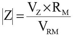
EQUATION 3.
To find the phase angle, use the current (I∠0) in Rm as reference and plot the three voltages VRM, Vz, and Vs as shown in Figure 4 for some arbitrary Z.
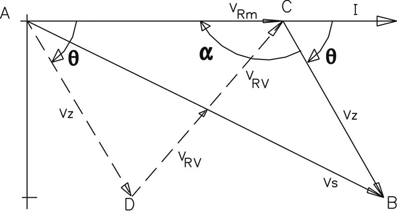
FIGURE 4. Phasor diagram for circuit.
The angle θ is the angle of Vz with respect to VRM and is also equal to (180 - ∠α ) degrees. Cos(α) can be found from the law of cosines for triangle ABC. After some algebraic manipulations, cos(θ) is found in terms of the voltage magnitudes as shown in Equation 4:
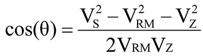
EQUATION 4.
We see from Equation 3 that the impedance calculation depends critically on the value of Rm, so it must be known precisely. But, as seen from Equation 4, the method is not able to distinguish the sign of the angle, since the cos(θ) = cos(-θ), so we must use other means to determine if the measurement is inductive or capacitive. Ways for doing this are discussed later on.
If we have a good AC voltmeter that can measure voltages without loading the circuit, all we need to do is measure the voltages shown and apply them to Equations 3 and 4. We also need a hand calculator, using the inverse cosine function, to find θ from the result of Equation 4. In the old days when measurements were made on 60 Hz power systems, this worked fine. But if we want to work in the high frequency range, most digital AC voltmeters won’t measure AC voltages properly. Since the majority of us do not have a good RF, high impedance AC voltmeter, we will need another method of obtaining the voltages. A simple way of doing this is presented later on.
Before we leave this subject though, it should be mentioned that the SWR and reflection coefficient at the load can be calculated once Z∠θ is found. In this case, the reflection coefficient r can be found from:
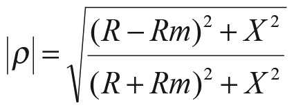
EQUATION 5.
Here, R and X are the resistive and reactive parts of Z. The SWR can be found from:
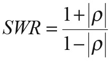
EQUATION 6.
Note, too, that the reverse voltage VRV shown in Figure 3 can be calculated from the three original voltages measured even without the two resistors R1 and R2 being present. To see this, refer to Figure 4 and note the triangle ADC where Vz and VRV are shown dashed. The vector VRV + VRV goes from D to C and bi-sects Vs, if we assume R1 = R2. On the other hand, if we physically add the two resistors R1 and R2 to the circuit, we can measure VRV and calculate VS. This provides us with an alternate set of three voltage measurements and provides for the calculation of cos(θ) by means of another equation. This equation can be found by applying the law of cosines to triangle ADC to find cos(θ) from Equation 7 as shown below:
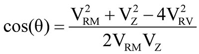
EQUATION 7.
The implications of this will be discussed in the next section.
Understanding Accuracy and Phase Errors
The TVM produces a reasonably good result for the magnitude of the impedance (see Equation 3) since we should be able to measure the two voltages Vz and VRM fairly accurately and Rm is known precisely. Impedance errors will occur when either Vz or VRM is very small, corresponding to large or small load impedances in which case the accuracy will suffer. Impedances near 50 ohms (where the voltages are roughly the same) and below an SWR of about 4:1 should be calculated fairly accurately.
Calculation of the cosine of the impedance angle θ is another story. Theoretically, Equations 4 and 7 would produce identical results. But practically speaking, there will be a difference depending upon the load impedance. What must be realized is that in a practical circuit there will be measurement errors and they will affect these two equations differently. Below is a numerical example to illustrate. More general comments follow the example.
Consider, as an example, a circuit such as shown in Figure 3, where R1 = R2 and Z = Rm = 50 ohms (corresponding to an SWR of 1:1 at the load Z). Assume the measured voltages are VRV = 0.000 V, VRM = 1.000 V, VZ = 1.000 V, and VS = 1.999 V (which has a negative error of 1 mV) since VS would equal 2.000 volts in a system with SWR of 1:1. Calculating from Equation 4 yields cos(θ) = 0.998 while Equation 7 yields cos(θ) = 1.000 as it should. So, we have incurred an error of 0.2% with the first calculation and an error in the angle of 3.6 degrees but there was no error with Equation 7.
Note, too, that the error can conspire to make the cos(θ) >1, which is theoretically impossible for the cosine function. To illustrate, consider the above case with VS = 2.001 V (a positive 1 mV error) and calculate cos(θ) from Equation 4 as 1.002.
Now consider the same example except that VRV = 0.005 V (a positive 5 mV error) and VS = 2.000 V (no error). Calculation from Equation 4 yields cos(θ) = 1.000 while Equation 7 yields cos(θ) = 0.9999. So, we have incurred only an error of 0.01% with the second calculation and an error in the angle of 0.81 degrees but with an assumed, much larger, measurement error.
Clearly then, as shown above, Equation 7 is less sensitive to errors for this particular case of a resistive load. Of course, this is not rigorous proof, but other examples at higher SWRs show a similar advantage. The author has performed a sensitivity analysis of cos(θ) with respect to VRV and VS in Equations 4 and 7, respectively. Sensitivity analysis refers to the sensitivity of a circuit parameter or value to errors in the component or some other value such as voltage. The mathematical details are too long to present here, but the results show that Equation 7 has the least sensitivity to errors when the load is resistive and at low SWR. Therefore, the circuit based on Equation 7 is chosen.
I hope that from the above discussion you can appreciate the importance of accurate measurements. As a further illustration, consider using an eight bit analog-to-digital converter (A/D) to measure the voltages in the above numerical example. Since we have a maximum voltage of two volts and 256 levels with an eight bit unit, each level corresponds to 7.81 mV. Clearly, only a one level mistake may cause a moderate angle error. On the other hand, modern digital multimeters have counts (levels) ranging from 2,000 to over 50,000 and 3-1/2 or more digits with 0.5% or better accuracy. This should provide a fairly economical and accurate means of collecting the voltage data. (More details are discussed later on.) Now let’s take a look at how to measure the voltages required with an ordinary digital multimeter.
Diode Sampling Circuit
A circuit that is commonly used to convert AC voltages to DC for measurement is the “diode voltage sampler” (DVS) shown in Figure 5.
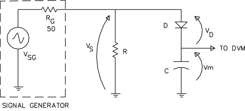
FIGURE 5. Diode voltage sampler.
In this case, we want to find the voltage VS across R. Here’s how it works. The positive, peak AC voltage across R is rectified by diode D and charges capacitor C. Once the capacitor is charged to about the peak value of VS, it no longer places a load on R except for the minute amount of current needed to keep it charged. A high input impedance DVM can read the voltage on C which should be close to the peak value of VS.
Of course, for maximum accuracy, we should add the value of the diode voltage drop VD to the DVM reading Vm. If VS is large, the diode drop is often neglected or considered a small constant of say, 0.7 volts, for a silicon diode. And as long as the diode voltage drop is small compared to VS, this works reasonably well. But if VS is smaller, say, 1.5 volts peak, the diode drop needs to be estimated better. And for even smaller voltages — as we might find in our impedance measuring circuit — it becomes critical to know the exact value of the diode drop to compensate our DVM reading.
A method that I have used with some success employs a mathematical model of the diode in the PC software. Knowing the diode parameters enables better compensation by using the model to estimate the diode voltage drop. Unfortunately, it is not perfect as it still leaves room for error due to manufacturing tolerances and capacitance effects. These errors can be ameliorated somewhat by calibrating the model with known impedances at specific power levels.
To see how the diode compensation works, refer again to Figure 5. Recall that the objective is to find an estimate of VS from a measurement of Vm. This is done by estimating the diode voltage drop, VD, and adding it to Vm, to form the estimate of VS. To find VD, consider the diode equation below:
EQUATION 8.
Solving for VD yields:
EQUATION 9.
where N =1, VT = 26 mV @ 25°C, IS = 22.31 x 10⁻⁹ A and ID is the diode current, according to the Agilent Spice model on the 1N5711 datasheet. So, everything is known except for ID which can be approximated by Vm/Req where Req is the equivalent impedance of the DVM or other resistive loads on the diode that we may add later. Since Vm is measured and Req is estimated, this is a good starting point to find ID and, therefore, VD. A better estimate for the diode voltage drop can be found by adjusting Req under known conditions such as a specific power level and known resistive load. More details on the calibration using known resistors is discussed later on.
Another thing we can do to improve accuracy is to employ a fast switching diode that does not conduct substantially after the peak voltage has passed as that would reduce the capacitor voltage. Diodes meant for 60 Hz power supply use are not usually built for speed, and shouldn’t be used in an RF peak detector. A Schottky diode (or barrier diode) like the SD101A, 1N6263, or 1N5711 are better options and also produce a low voltage drop. Germanium diodes like the 1N34 also have a low voltage drop but are prone to temperature and matching problems. I have found the 1N5711 to be a good choice and it is available from many sources for around $0.30 each.
Another effect that is hard to compensate for is the diode capacitance. For the 1N5711 model, the package capacitance can be 2 pF, which causes some bypassing of the AC signal around the diode. At 14 MHz, this bypass impedance can be as low as 5,600 ohms. Measurements made on the above sampler with a DC multimeter confirmed that the measured voltage tends to fall off with frequency.
The TVM circuit can be modified by adding a DVS across each resistor that has an AC voltage that we wish to measure. If the resistances are low enough (in the 50 ohm range) and the input impedance of the DVM is large enough, the basic circuit operation will not be affected substantially. To confirm this, I viewed the AC voltage across a 100 ohm resistor (in a circuit similar to Figure 5) with a Tektronix TDS360 digital oscilloscope when driven by a Wavetek Model 81 signal generator at 3.5 MHz.
No visible difference in amplitude was seen when the sampler was placed across the resistor. But what surprised me was that the scope probe (10 Meg and 15 pF) affected the voltage read by the DVM slightly, probably due to the probe capacitance. So, don’t leave any probes connected to the circuit during impedance measuring!
There are a number of ways that the samplers can be added to the circuit of Figure 3. After considering several possible variations and testing for accuracy, the circuit shown in Figure 6 emerged as the best and was chosen for the final implementation.

FIGURE 6. Three voltmeter circuit with diode samplers.
RF Impedance Analyzer Circuit
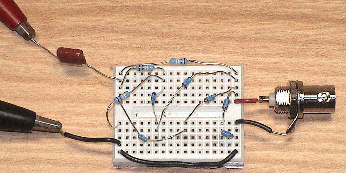
Figure 7 shows my breadboard setup for the impedance analyzer. A BNC connector (shown on the right) is used to connect to the load Z. In this instance, I am using a solderless breadboard as it is an easy way to get started and confirm operation of the circuit. However, be aware that I am not recommending this construction method as it is limiting in terms of stray capacitance between components and has no shielding. Even though I used triple spacing between components on the breadboard, I started noticing frequency effects above 10 MHz.
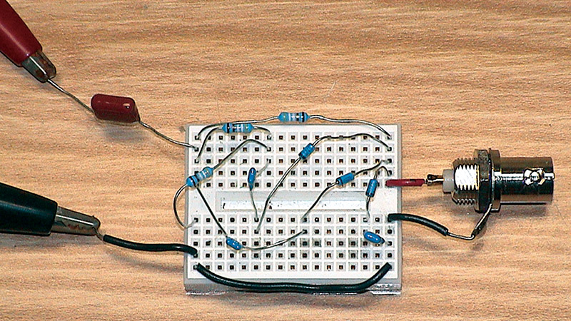
FIGURE 7. Photo of breadboard setup of the impedance analyzer.
Placing the circuit on a PCB (printed circuit board) with parts spaced apart and inside of a metal enclosure with the appropriate connectors and switch should be a better option. Actually, it shouldn’t be too complicated to build and it should make a nice weekend project as it is straightforward and there is no power supply needed.
Now, refer again to the impedance analyzer circuit schematic shown in Figure 6. Only a few parts are required but they must be selected carefully for best results. D1 through D3 are 1N5711 Schottky diodes. It is best if they are matched. I bought 10 diodes which were packaged on a tape reel and chose three diodes that were placed together. Of course, this doesn’t guarantee the diodes are matched, but it may improve the odds. Similarly, I bought 20 pieces of 49.9 ohm, 1/4 W, 1% resistors and carefully measured each one. I found one that was 50 ohms and used that for Rm.
I also found several resistors that were close to 49.8 ohms which were then used for R1 and R2. It is important that these two resistors be matched in value. I also matched the three capacitors C1 through C3, 390 pF, 5% ceramic capacitors which should be COG type. I also purchased some 12.5, 25, 100, and 199 ohm, 1/4 watt, 1% resistors for use in calibration.
Shown on the diagram are a coupling capacitor C4, a switch SW1, and filter components R3, R4, and C5. Tolerances of these components are not critical. R4 may or may not be required, depending on the input impedance of your DVM. This is discussed in more detail later on. SW1 is used to select the voltage for measurement by the DVM. Finally, you should choose the appropriate input and output connectors for the type of measurement you will make, be it a component or transmission line.
Signal Generator and Digital Multimeter Requirements
A sine wave signal generator with 50 ohm output impedance that produces a reasonable level is needed. Signal generators are usually rated in dBm output (for 50 ohm systems) which can be converted to peak volts, as needed. For example, 13 dBm output into 50 ohms produces 1V RMS, or about 1.414 volts peak. Although the generator will not always see 50 ohms, this is still a convenient reference point. Because of the diode nonlinearity, there is a lower limit of generator output where it becomes very difficult to compensate accurately for the voltage drop. This occurs somewhere around 13 dBm. I don’t recommend using a generator with an output below this value.
Unfortunately, some generators “max” out at 10 dBm (0.707 VRMS or one volt peak) and would produce marginal results. Several generators in my shack have that limitation. On the other hand, many generators can produce much more. My Wavetek Model 81, 50 MHz generator can produce up to 24 dBm (or five volts peak voltage).
Some generators produce a DC offset voltage which can cause the diode sampler to have an error. My Wavetek — although it was set for 0 volts offset — actually produced 6 mV offset, and while that doesn’t sound like much, it was enough to cause errors. I cured the problem by placing capacitor C4 in series with the generator to block the DC voltage.
A QRP rig is probably over-powered for use as a signal generator for this application, so an attenuator must be used to bring the level down below 24 dBm. Attenuation of transmitters is beyond the scope of this article so you will need to consult an appropriate radio handbook.
Digital voltmeters or multimeters are very common today. A basic DC accuracy of 0.5% or better is needed. Normally, when accuracy is specified in this manner it means 0.5% of span. So, if your voltmeter range or span is, say, two volts, then an error of 0.5% of two volts (plus or minus 10 mV) is still within specifications.
Of course, it doesn’t mean you will necessarily see that large of an error. Many of the very low cost units are definitely not appropriate as they are rated above 0.5%. Some economical units can be found with an accuracy better than this. Unfortunately, a few meters may proclaim high accuracy but it may well be salesmanship on their part. Caveat emptor!
Multimeters can have quirks. As a case in point, an auto-ranging digital multimeter, with a stated accuracy of 0.3%, was obtained on the Internet for around $19. With the range fixed, it produced acceptable results but when in auto-range mode, produced errors as high as 40% on low voltages. Why? As it turns out, for the lower DC range, the meter’s input impedance changes from 10 Meg-Ohms to over 100 Meg-Ohms. This causes a different loading on the circuit in Figure 6, with resulting higher voltages measured on the low range. This can be remedied by fixing the range so that it is not allowed to auto-range to the lowest span. This seems to work best with meters having higher counts.
Even high-end meters like the Protek 608 have different input impedances for different ranges. For example, on the 500 and 2,500 mV ranges the input impedance is greater than 1 Giga-Ohm. On the 5.0 to 5,000 volt ranges, the input impedance ranges from 10 to 10.5 Meg-Ohms.
If the input impedance is extremely high, looking at a capacitive load like C5 in Figure 6 may cause problems, so resistor R4 was added. It may not be needed in some cases, and if omitted, will allow a higher voltage to be measured. Note, too, that some DVMs have a low input impedance and are designed for special applications. An input impedance of at least 10 Mohms is needed here to prevent over-loading the diode voltage samplers. Be sure to check your meter for accuracy, try to avoid changing ranges, and watch out for auto-ranging mode.
For the record, four DVMs were tested in this project. They included a Kelvin 200LE (2,000 count, 0.5%), Gardner Bender GDT-193A (2,000 count, 0.5%), Circuit Specialist MY-68 (3,260 count, 0.3%), and a Protek 608 (50,000 count, 0.05%). The first three are low cost meters and produced acceptable results with the Protek producing slightly better results. I believe the calibration routine (discussed later) helps fine-tune the results for a specific meter and improve accuracy. So, if you change meters, you probably should re-calibrate the software.
RF Impedance Analyzer Software
The impedance analyzer software is available in the downloads at the end of this article. When you’re ready, unzip the software to a new folder and run the executable (exe) program. It was tested with Windows 98 and XP. When you run the software, you may get a message like “Required DLL file MSVBVM60.DLL was not found.” This is a Visual Basic run time file and is on many systems. If not found, you will need to obtain it and install it on your system. It is freely available from Microsoft and other sites on the web. It is usually available as Visual Basic 6.0 SP5: Run-Time Redistribution Pack (VBRun60sp5.exe) and is a self-extracting file. Download takes about six minutes at 28.8 kbps.
If you get the message “Component ‘COMDLG32.OCX’ or one of its dependencies is not correctly registered: a file is missing or invalid.” when you try to run the program, you will need to register it on your system. It is also freely available from Microsoft and other sites on the web. More details are included with the software.
If you just want to experiment with the impedance analyzer program, go ahead as it does not modify the registry or install any other material on your computer. You can remove it by just deleting the entire folder it is located in.
A screenshot of the main screen of the impedance analyzer is shown in Figure 8. It is easy to use. Just enter the measuring frequency and the three voltage measurements you obtained from the circuit into a single row. Up to eight rows of data may be entered so that you can get a better picture of how the impedance varies with frequency.
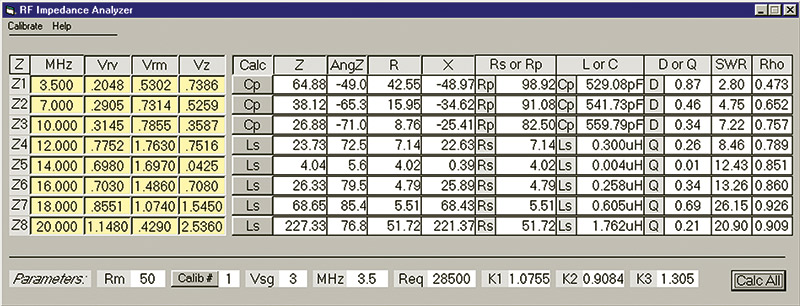
FIGURE 8. Main window of the RF impedance analyzer program.
To see the result for a row, click the “calculate” button in that row. That button also cycles through the Ls, Cs, and Cp options so you can view the results for different circuit models as discussed previously. The Lp model was not implemented as it is seldom used. You can also click the “calculate all” button at the bottom of the screen, if you wish to calculate all of the rows of entered data at one time. To get maximum benefits from the program, it should be calibrated as discussed next.
Calibrating and Using the Impedance Analyzer
The parameters the program will use when the “calculate” button is clicked are displayed near the bottom of the main screen. These values correspond to Rm and the diode models used in the circuit. Parameters need to be changed since, when you obtain the program, they will correspond to the Rm and diodes in my circuit.
To get the proper values for your diodes is easy, and a calibration method using four resistors is part of the program. I have found that good results are obtained if you use two resistors above 50 ohms and two below 50 ohms. I use the values of 12.5, 25, 100, and 199 ohm (1/4 watt, 1% resistors) to get an SWR of about 4:1 above and below the 50 ohm nominal value. This gives maximum accuracy in this range of SWR. You don’t need to use the same values as I did, but you do need to be able to measure them as accurately as possible for the program.
Now click “calibrate” at the top of the screen and a new window will open up as seen in Figure 9 with boxes for you to enter the resistor values and the corresponding measurements for each one. Let your equipment warm up for a few minutes before measuring and do it as accurately as possible. Include data on the measuring frequency and voltage level of the signal generator VS so it can be saved with your measurement data. Then click the “calibrate” button and wait while the program calculates the best diode parameters for your application.
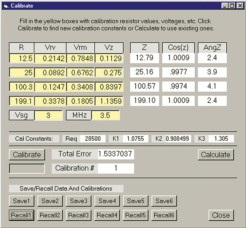
FIGURE 9. Calibration window of the RF impedance analyzer program.
When finished, the right side of the screen shows the calculated impedance magnitude (which should be close to the resistor values) and the angles (which should be less than 6 degrees). When done, be sure to save the calibration using one of the buttons on the bottom. You may wish to provide other calibrations for different power levels or frequencies.
Up to six calibrations may be saved. These can be called up from the main screen. Calibration data is saved in a file RFinit upon exit. My data is in the original file so you can see my resistor values, voltages, and calibration results. When you save your data, it will just overwrite the old data.
There is a quirk with the TVM calculation as alluded to earlier whereby the result of the cosine calculation may produce a value greater than one. This happens only with resistors where the phase angle is supposed to be zero. Slight inaccuracies in measurement are the cause of the problem. To keep you informed of this situation, the results of the cosine calculation are shown on the calibration screen. Don’t be alarmed if you see cosines above one. Hopefully, they will be very close to one and won’t affect the program results substantially. This is just a peculiarity of this method.
On the main screen, the box with the offending angle (cosine greater than one) will be highlighted in a red color. Since the error is often small and occurs mainly with resistors, the program will substitute a suitable small angle. In case you don’t like the value chosen, you have the option of assuming the angle to be zero. Also, if you don’t like the calibration values found by the computer algorithm, you can try to adjust them manually. The resulting error is shown on the screen as a guide. I have tried several times to “best” the program but have been unsuccessful. It seems to do a good job, though.
The calibrate algorithm is straightforward. An error criterion shown below is evaluated by a brute force search for the minimum of “Error.” Each diode parameter is varied separately in tiny increments and “Error” calculated.
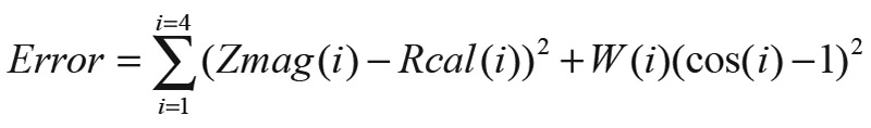
EQUATION 10.
Here Zmag(i) is the calculated magnitude of Z, Rcal(i) is the calibration resistor, W(i) is a weighting factor on the cosine error, and “i” is the first through fourth calibration resistor. The first term in the sum is the error due to magnitude error or the difference between the calculated Z and the calibration resistor. The second term is the error between the calculated cosine and the value of one, which it would be for a resistor. The weighting factor W(i) is set to 10,000 since the cosine changes are small and change slowly near one.
The algorithm stops when it can find no variation in the diode parameter that reduces “Error” any further. These parameters are shown on the screen. This doesn’t necessarily mean the lowest error is found. There may be other local minima due to the nonlinear property of the diode and there is a possibility that the algorithm has gotten stuck on one of these. But as noted above, I haven’t been able to find a better minimum in my testing.
Determining the Sign of the Impedance Angle
We saw previously from Equation 4 that the analyzer cannot determine the sign of the impedance angle, θ, so let’s explore other methods of finding it.
For lumped parameter components like capacitors and inductors, the sign is obvious since capacitive reactance is negative while inductive reactance is positive, as seen in Figure 1. This leads to the following simple rule of thumb for lumped parameter parts.
If |Z| increases with increasing frequency, then the load is inductive and θ > 0. While if |Z| decreases with increasing frequency, then the load is capacitive and θ < 0. So, by slightly changing the frequency and looking at the change of impedance, we can find the sign. This rule works for RC and RL circuits and even simple RLC circuits. An easy way of doing this is to monitor Vz. For example, if Vz is decreasing as frequency increases, the load is capacitive.
If we look at the input impedance of a transmission line with a load attached, the above rule is not strictly obeyed. It may be obeyed at some frequencies but not at others. There is a special case where it is obeyed — that of a zero resistance load — an example of which will be discussed later on. But in general, the rule does not hold, particularly if the load is complex. So, if you are not sure of the nature of the load attached to the transmission line, do not use the above rule.
There are other ways of finding the sign. It is an easy matter to add a small amount of reactance in series with the input and observe the angle change. For example, if you added some capacitive reactance and the angle increases, then the input is capacitive and the angle is negative.
If you know the length and type of transmission line and the type of load (such as an antenna), you can make some good estimates of the sign. For example, if the load is an 80-meter dipole of known resonant frequency, you can expect the antenna to be capacitive just below resonance and inductive above resonance. Then using a program like AC6LA’s Transmission Line Details (TLD), you can calculate an estimate of the input impedance which should help determine the sign. TLD is designed for Windows and easily found on the web [3]. Let’s look at some other applications.
Applications of an Impedance Analyzer
Uses for an impedance analyzer abound. And if the accuracy requirements aren’t extreme, this unit can produce good results. It can be used to check components like inductors and capacitors at their operating frequency, measure the input impedance of a matching network, and even measure the impedance of an antenna. Coaxial cable transmission lines — which often seem mysterious to many — can be investigated easily with this analyzer.
First, let’s consider a simple RC circuit consisting of a 100.3 ohm resistor and a 527 pF mica capacitor connected in parallel. The component values were individually measured at an audio frequency of 1 kHz. I connected them in parallel as the unknown Z for the analyzer, read the three voltages at 3.5 MHz, 7.0 MHz, and 10 MHz, and entered the data into the program. Figure 10 shows a comparison of the measured and theoretical values.
| Impedance Measurement of Parallel RC Circuit |
| |
Theoretical |
|
| Frequency |
Z∠θ |
R + jX |
D |
SWR |
Rp |
Cp |
| 3.5 MHz |
64.9 -49.2 |
42.6 -j49.5 |
0.86 |
2.8 |
100.3 |
527 pF |
| 7.0 MHz |
39.6 -66.8 |
15.6 -j36.4 |
0.43 |
5.0 |
100.3 |
527 pF |
| 10.0 MHz |
28.9 -73.2 |
8.4 -j27.6 |
0.30 |
7.9 |
100.3 |
527 pF |
| |
Measured |
|
| Frequency |
Z∠θ |
R + jX |
D |
SWR |
Rp |
Cp |
| 3.5 MHz |
64.9 -49.1 |
42.5 -j49.1 |
0.87 |
2.8 |
99.1 |
529 pF |
| 7.0 MHz |
38.5 -65.4 |
15.9 -j35.0 |
0.46 |
4.7 |
92.5 |
537 pF |
| 10.0 MHz |
27.3 -70.9 |
8.9 -j25.7 |
0.35 |
7.1 |
83.3 |
551 pF |
FIGURE 10. RC circuit test results compared to theoretical values.
Notice that at 3.5 MHz, the accuracy is very good although the SWR is over 2:1. As the frequency increases, and the SWR does too in this case, we see an increasing difference between the measured and theoretical values of the angle and magnitude. This translates to different values for the computed Rp and Cp components.
The increasing difference as the frequency climbs is probably due to several factors, including stray capacitance of the breadboard, long leads on the components, dissipation in the capacitor, diode modeling errors, and high SWR, in the last case, of over 7:1. This example should give you an idea of what to watch out for and what you can expect.
For the next example, consider measuring the impedance of a long wire antenna. To create the antenna, a spool of wire was unwound and strung out over the floor with a length of about 34 feet. This is close to one-quarter wavelength for the 40 meter ham band and should resonate near 7.0 MHz. One end of the wire was connected to the analyzer and the remainder, on the far end, left on the spool. While carefully tuning the signal generator frequency, VRV was monitored with the DVM until a dip was found. This occurred near 6.8 MHz.
The antenna is expected to be capacitive below this frequency and inductive above it. Impedance measurements were then made at frequencies from 6.6 to 7.1 MHz. Figure 11 shows the results of the measurements along with those taken with a commercial RF impedance meter. The TVM analyzer data is shifted slightly in frequency, probably due to a small amount of stray capacitance. Otherwise, the TVM RF analyzer does a respectable job compared to the commercial unit.
| Frequency |
Comm. Analyzer |
TVM Analyzer |
| 6.6 MHz |
79.1∠-21.9 |
76.9∠-26.9 |
| 6.7 MHz |
73.9∠-13.2 |
73.1∠-16.5 |
| 6.8 MHz |
69.7∠+0.6 |
72.6∠-7.7 |
| 6.9 MHz |
73.9∠+14.2 |
74.6∠+11.1 |
| 7.0 MHz |
80.0∠+23.2 |
83.9∠+17.7 |
| 7.1 MHz |
88.9∠+31.9 |
93.0∠+27.4 |
FIGURE 11. Impedance of 40 meter long wire antenna.
As a more complex example, consider a long piece of RG58 coax of unknown length that was pulled out of my junk box. We know that if the cable is 1/2 wavelength long, it will reflect the load impedance back to the input. So, initially we need to find the frequency corresponding to this length. This is easily done with the analyzer.
We start by making the load impedance of the coax a short circuit. This will reflect a small, nearly zero impedance back to the input at the 1/2 wavelength frequency. To find this point, we connect the analyzer to the input and vary the frequency while monitoring Vz for the lowest voltage. In my case, this occurred at 13.9 MHz. See Figure 12 for the test setup.
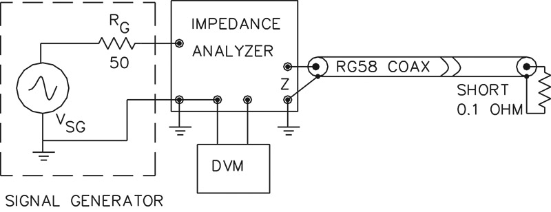
FIGURE 12. Setup for checking coaxial cable with analyzer.
Next, I wanted to find the physical length and the input impedance of the cable at other frequencies. A coaxial cable with a short on one end presents a wide variety of input impedances that go from nearly pure capacitive to resistive to inductive and back to capacitive again, repeating the cycle over and over with frequency. As such, it makes an ideal test subject. But be warned, the impedances can extend into the thousands of ohms at some frequencies — well beyond the range of the analyzer.
Fortunately, there are programs available on the Internet to find the length and calculate the theoretical impedance given the 1/2 wavelength frequency. A good choice is the previously mentioned TLD. Given the load impedance (shorted in this case), it will calculate the theoretical length and input impedance of the cable at other frequencies. These values can then be compared to the values obtained by the analyzer and give us an idea of how well the analyzer performs. By the way, for a loss-less cable with a resistive termination (including a short), the above rule of thumb for finding the sign does hold. This is easily seen using TLD.
The cable manufacturer wasn’t known, so Beldin was assumed. The cable data (RG58 Beldin 9201) and 1/2 wavelength frequency were entered into TLD and the physical length calculated as 23.35 feet. The load (short resistance) was assumed to be 0.1 ohms with zero reactance. Next, a number of frequencies were entered into TLD and the theoretical input impedances predicted. This data along with selected, actual measured values obtained with the analyzer are shown in Figure 13.
| |
TLD Calculated |
TVM Analyzer |
| Frequency |
R + jX |
Z |
R + jX |
Z |
| 5.0 MHz |
6.8 + j110 |
110 |
6.8 + j115 |
115 |
| 6.0 MHz |
29.4 + j234 |
237 |
30.2 + j240 |
242 |
| 8.0 MHz |
27.7 – j211 |
213 |
38.5 – j213 |
217 |
| 10.0 MHz |
4.3 – j63 |
16 |
8.9 – j63 |
64 |
| 12.0 MHz |
2.3 – j23.9 |
24 |
5.5 – j23.5 |
24 |
| 14.0 MHz |
2.1 + j1.2 |
2.3 |
3.3 + j1.7 |
3.5 |
| 16.0 MHz |
2.8 + j26.7 |
27 |
4.6 + j28.1 |
28 |
| 18.0 MHz |
6.4 + j68.8 |
69 |
6.1 + j67.9 |
68 |
| 20.0 MHz |
63.0 + j251 |
259 |
52.0 + j216 |
222 |
FIGURE 13. Coaxial cable test results of shorted cable.
As shown, the values are reasonably close. Don’t assume all of the differences are due to errors of measurement of the analyzer. The theoretical calculations don’t take into account connectors, the effect of splices (my cable had one), and age factors of the cable. In this case, I appreciate the confirmation of the closeness of the data but tend to lean to the actual measurements as being more true.
As an interesting experiment, if you connect an antenna to the coax as a load (replacing the short), you can again measure the input impedance at some frequencies of interest. Using TLD (in reverse), should then enable you to find the impedance at the antenna. This obviates the need to go directly to the antenna for measurement.
Final Comments
The straightforwardness of the impedance analyzer makes it attractive as a low cost measuring tool. But, belying this simplicity, there are limitations on its accuracy at low impedance angles and at high SWR. It certainly won’t replace a good network analyzer, so don’t sell your stock in Agilent!
On the other hand, it can be very useful in many situations where a more sophisticated instrument is not available. Accuracy is good over a reasonable impedance range of about 5 to 1,000 ohms, and better between 10 and 250 ohms. Angles near zero degrees (corresponding to a pure resistive load) and angles near 90 degrees (corresponding to a pure reactive load) are the least reliable. Making manual voltage measurements and entering them into a program may seem like a drawback to some, but I have found it to be surprisingly easy to do and very informative in many cases. I was often amazed by the analyzer’s accuracy and seldom dissatisfied with it. Overall, it works well if you understand its limitations. If you find yourself making lots of measurements or needing more portability, you may want to consider moving on to a commercial impedance analyzer.
It was fun and instructive working with this impedance analyzer. I hope you will find that to be the case, too. So angle for some time, analyze your resources, and don’t be impeded in building your own version! NV
References
[1] George Steber, “A Low Cost Automatic Impedance Bridge” QST, October 2005, pp 36-39.
[2] George Steber, “LMS Impedance Bridge” QEX, Sep/Oct 2005, pp 41-47.
[3] Transmission Line Details, Dan Maguire AC6LA, available free as a download at www.ac6la.com.
Downloads
Impedance Analyzer Software