DFT Basics

---

For some electronics hobbyists, the discrete Fourier transform, or DFT, is a feared and mysterious entity that is best left to the “experts” or those who practice in the field of digital signal processing (DSP) on a daily basis. The truth is, however, that with a little explanation and only a dash of simple math, anyone who can use a spreadsheet or program a microcontroller can understand and put this powerful signal processing technique to work in no time at all.

For those who have never heard of the DFT before, here’s a little background. Every signal can be viewed in at least two ways. The most common way is in the time domain. Whenever we look at a signal on an oscilloscope, we’re seeing it in the time domain (the X axis is time). However, we can also view a signal in the frequency domain, so that as we move along the X axis in the positive direction, we’re looking at increasing frequency. The Y axis represents the amplitude of the frequencies. It should be noted that these two domains are like opposite sides of the same coin. One cannot exist without the other, and both are equally valid.

Why bother with the frequency domain? Without going into the mathematics, let’s just say that some problems are more easily solved by converting a signal to the frequency domain first, doing some math, and then converting the solution back to the time domain. Examples are readily found in communications where signals are often mixed (heterodyned) and modulated in different ways. Multiplication of sines and cosines can be quite cumbersome in the time domain, but more easily managed in the frequency domain.

Let’s look at a sample signal in both domains. If we were to add a 200 Hz sine wave (amplitude 1), a 600 Hz sine wave (amplitude 1/3), and a 1,000 Hz sine wave (amplitude 1/3), we would get the signal in Figure 1a.

FIGURE 1a. Signal in the time domain. The X axis is time.

---

To most people, it would not be obvious that these three frequencies are present in the figure. However, decomposing the signal in Figure 1a into its frequency components clearly shows which frequencies are present and at what amplitude (Figure 1b).

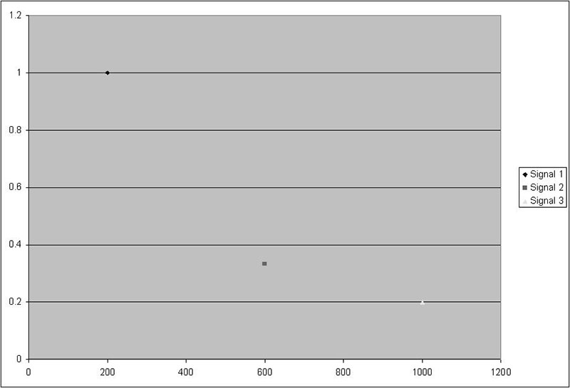
FIGURE 1b. Signal in the frequency domain. The X axis is frequency.

---

This example hints at another very important concept: All (reasonably continuous) signals can be made up of a combination of sines and/or cosines. This is Fourier’s theorem. You can experiment with this idea using the “Synthesis” tab in the “dft.xls” spreadsheet available in the downloads.

Here’s a question for you: If we’re given a signal in the time domain, is it possible to represent this signal in the frequency domain? In other words, can we go from something that resembles Figure 1a and determine the same kind of information that’s presented in Figure 1b? This answer is — of course — yes. One method of doing this is to use a discrete Fourier transform.

Let’s break down this exotic-sounding phrase into its basic parts. First of all, a transform is just a word that has to do with taking information in one form and looking at it in another. A simple example is taking Eastern Standard Time and subtracting three hours. If I do this, I’ve just performed a transform from EST to PST. Fourier (pronounced FOUR-ee-ay) is the name of the French mathematician who contributed greatly to his field. Discrete (as opposed to discreet) means separate. So, instead of working on an analog (or continuous) signal, we’re only working with specific (digital or discrete) values of a signal taken at evenly-spaced intervals of time. If we’re going to use a computer or microcontroller, we have to use a discrete technique.

As you read through this article, be aware that this is not a leisurely read. If this is your first time experimenting with the DFT, you will need to have your sleeves rolled up and your brain focused. Our discussion will be about DFT theory and the Excel spreadsheets that you will be using to experiment with these concepts.

Also keep in mind that my purpose here is to provide only a general introduction to the DFT and to provide the boilerplate tools necessary to launch into an independent detailed study or microcontroller implementation.

Procedure

First, we’ll discuss correlation — the basic building block of the DFT. Then, we’ll extend correlation to sampled signals, which is necessary for microcontroller and computer applications. Next, a functional DFT program will be demonstrated in Excel with a simple application. Finally, I’ll wrap up with a quick overview of aliasing — a nasty phenomenon you’ll want to avoid.

Correlation

Loosely speaking, this is a number that represents how well two signals are matched. The higher the correlation (or greater the value), the better they match. Correlation is found by multiplying the respective elements of two sampled signals together and adding each product together. To make this clearer, see Figure sets 2a and 2b.

 

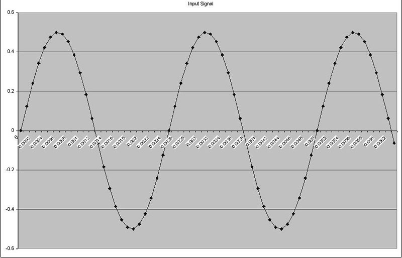
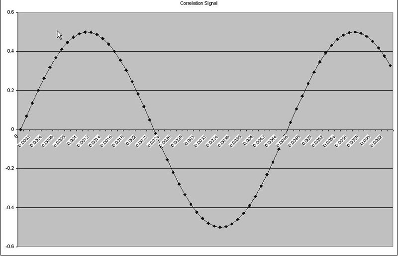
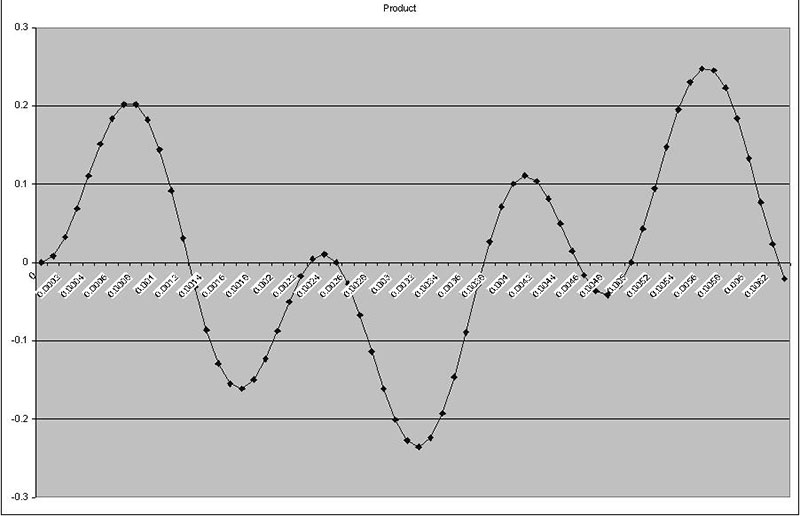
FIGURE 2a. These three graphs show signals with poor correlation.

---

Figures 2a3 and 2b3 are the products of the other two related signals. They contain points both above and below zero. So in summing the correlation, some points will be added and others subtracted. In Figure set 2b, the input and correlation signals are the same (2a1 and 2a2), so all of the points in the product signal (2a3) are greater than zero (remember, a negative multiplied times a negative is a positive).

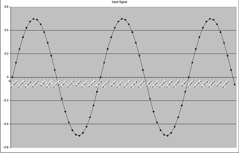
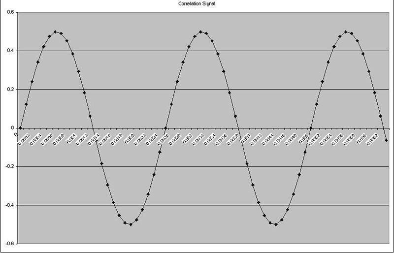
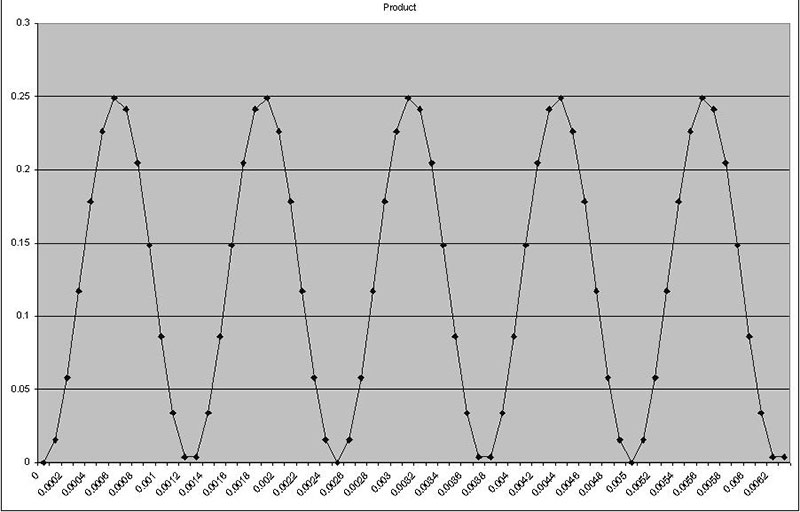
FIGURE 2b. These three graphs show signals with excellent correlation.

These plots were produced from the “Correlation 1” tab in the Excel spreadsheet. If anything up to this point is unclear, you may want to take a moment and experiment with this worksheet. You can see the cell formulas and change parameters of the test signals. The important concept here is that the closer two signals are to being “the same,” the higher the correlation.

Sampled Signals and Basis Functions

Figure 3 shows a signal that is identical to the signal in Figure 2b3.

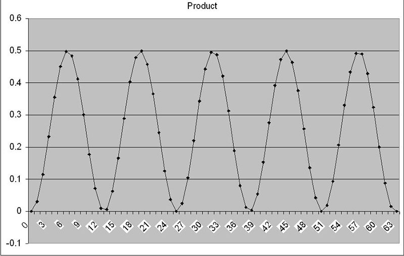
FIGURE 3. Sampled signal.

---

There is one very subtle and important difference in this graph, however. The units for the x-axis are not seconds but rather samples. When a computer or microcontroller takes A/D samples for the DFT, these values will be stored in an array for future processing. In the “Sampled Correlation” tab, there is an added column for sample numbers on the far left. Also in the worksheet is a parameter called “Basis Function.” This is a common name for the correlation signal.

The basis number is just the number of cycles of a sine (or cosine) wave that will fit in our sample size. The best way to see this is to put a few different numbers into the basis function cell and see the resulting signal. Figures 4a and 4b show a few examples.

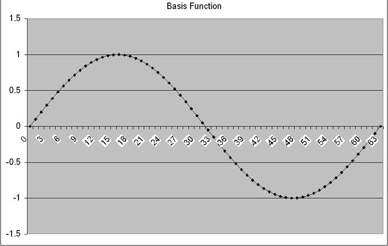
FIGURE 4a. Basis function = 1.

---

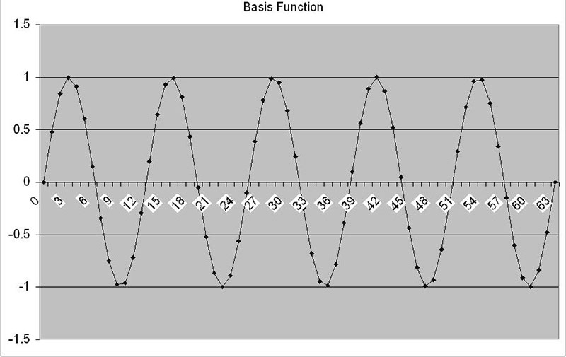
FIGURE 4b. Basis function = 5.

---

While it’s possible to put non-integer values into the spreadsheet, the DFT program we will use only uses integer values.

Performing the DFT

Here is where the fun begins (and may get a little complicated, so be patient). In the “DFT” tab, you can modify the test parameters to create a signal with a frequency, amplitude, and (DC) offset of your choosing. Once you’ve created a signal, press the “Perform Correlation by DFT” command button. This will execute a program written in VBA (Visual Basic for Applications) which you can view by going into design mode (this is done by pressing the “design mode” button in the control toolbar as shown in Figure 5 and then double clicking on the command button).

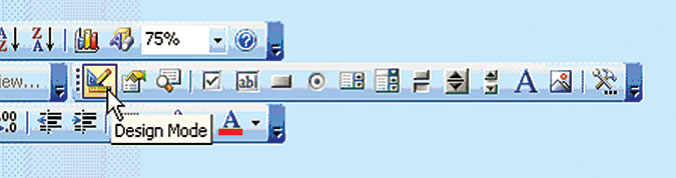
FIGURE 5. Entering and exiting the Design mode in Excel.

---

Executing the VBA code will result in two graphs being produced: the “raw” DFT, and the DFT corrected for sample frequency. Figures 6a, 6b, and 6c show an example with a test signal of 1,000 Hz.

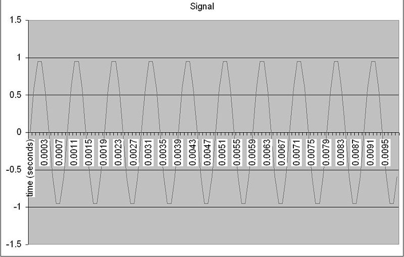
FIGURE 6a. Test signal.

---

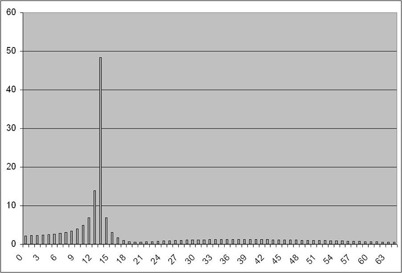
FIGURE 6b. “Raw” DFT.

---

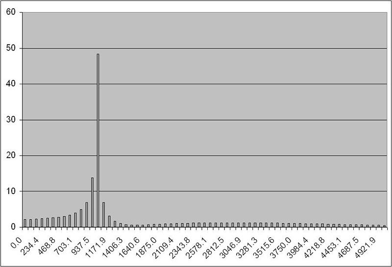
FIGURE 6c. DFT corrected for sample frequency.

---

Let’s take a moment and talk about what's going on in this short program. After initialization of variables and constants, the sample signal is read into the array “Sample.” Note that this is a 128 element array running from 0 to 127. So, our sample size is 128. Next, we initialize two 65 element arrays to zero. The purpose of these arrays is to hold the values of the sines and cosines that make up the test signal (see Figure 7). (For reasons we won’t go into here, cosines are referred to as the “real” part of the DFT while sines are the “imaginary” parts.)

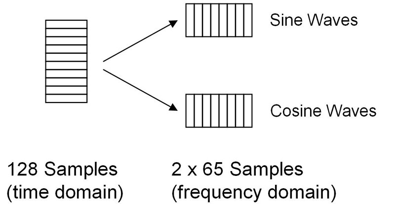
FIGURE 7. The 128 sample (time domain) array gets converted into two 65 sample (frequency domain) arrays.

---

Next, the test signal is correlated with sine and cosine basis functions. The correlation value with each basis function (remember, this is how “similar” two signals are to one another) is what gets stored in each element of the sine and cosine array. Finally, I merge the sine and cosine for each basis function into a root mean square value. This step is not really necessary, but I like to look at one final graph rather than two. If you prefer splitting sines and cosines apart, feel free to make two graphs. We’re not quite out of the woods yet, but we’re close. All that remains is to convert those 65 basis functions in each array into meaningful frequencies that we can understand. Remember, a processor is just crunching numbers in this DFT algorithm. It only sees samples, not voltages or frequencies. In order to convert to frequency, we multiply the sampling rate times the sample number and divide by the total number of samples.

Again, if any of this is unclear, look at the different Excel worksheets carefully. The cell formulas can be helpful. The “DTMF” worksheet demonstrates a useful application of the DFT. Instead of analyzing one signal, two can be broken down into their component frequencies and decisions can be made based on what is found.

Before wrapping up, there are a couple of items worth mentioning about the DFT.

Aliasing

You can only (reliably) sample signals with frequencies up to half the sampling frequency (called the Nyquist theorem). Sampling signals with higher frequencies will result in something referred to as aliasing. All this means is that the system is not sampling quickly enough to recognize the signal for what it is. In fact, the signal might be mistaken for something else.

To illustrate this, Figure 8a shows a 400 Hz sine wave. According to the Nyquist theorem, I need to sample this signal at a minimum of 800 Hz.

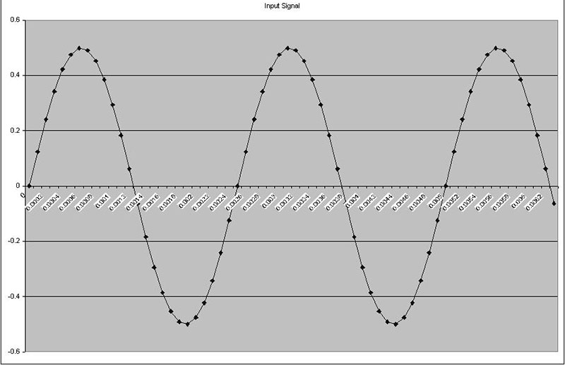
FIGURE 8a.

---

Figure 8b shows the 400 Hz signal sampled at a frequency of 3 kHz, well above the Nyquist rate. If you mentally connect the dots, you can probably make out the original signal without much trouble.

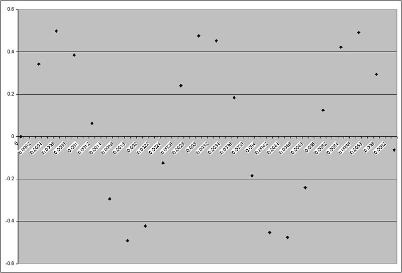
FIGURE 8b.

---

Figure 8c is our signal sampled at a 1 kHz rate, just a little above the Nyquist rate. While this may not look like a sine wave to you and me, it does to a DFT. Connecting the dots with a smooth curve may help bring out the original sine wave a little better.

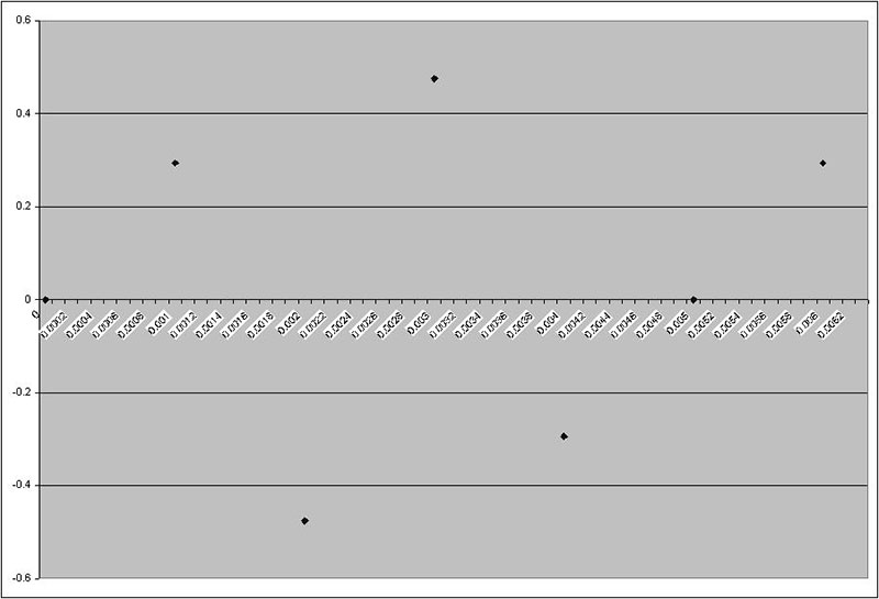
FIGURE 8c.

---

Finally, Figure 8d is the signal sampled at 500 Hz, which is below the Nyquist rate. Not only is the 400 Hz sine wave no longer discernable, but connecting the dots actually suggests a sine wave of a lower frequency!

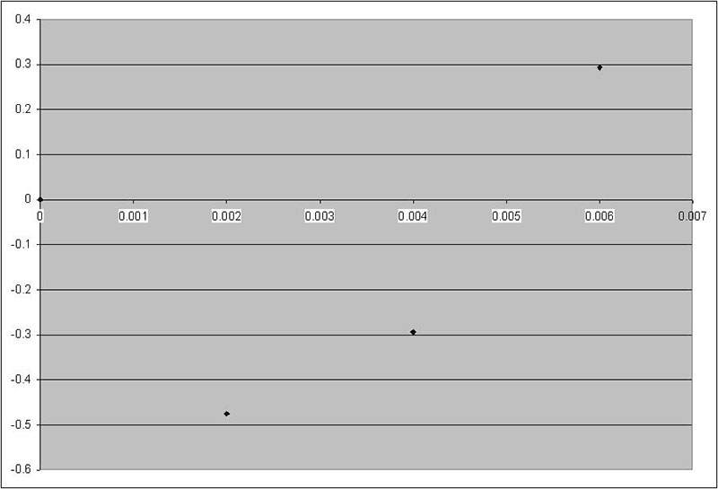
FIGURE 8d.

---

You can experiment with aliasing by going to the “DFT” tab and entering in a test signal frequency that is higher than half the sampling frequency (or lower the sampling frequency to get the same effect). You can also check out the “Aliasing” tab in the spreadsheet to see how I got these graphs.

DC Offset

There is one basis function that may not be obvious. Namely, a basis function with a frequency of zero. Not to worry, the DFT doesn’t miss this. The 0th element in each of the sine and cosine arrays contains the DC offset of the signal. Go to the “DFT” tab and try changing the test signal’s offset and see how that affects array element 0.  NV

---

---