Why You Need an Analog Front End and How to Set It Up

» Skip to the Extras

The analog input to an Arduino Uno has a resolution of only 10 bits. On a 5V scale, this is only about 1 mV of sensitivity. If you need more sensitivity, don’t look at another microcontroller. Look at adding an analog front end to your Arduino.

Singly or together, a general-purpose op-amp and an instrumentation amplifier — each operating on 0V to 5V power supplies — are the building blocks to an analog front end to any microcontroller. Here’s a practical way you can turn your Arduino into a high performance sensor measuring instrument.

Physical Computing

An Arduino is about as smart as a fruit fly. I base this on the gate count of the Atmel AVR 328 microcontroller — the brains of the Arduino board — which is a little less than 100,000 gates, including the 32K of memory and all the registers. A fruit fly has 100,000 neurons.

Just as the brain of a fruit fly processes sensory input information about the world around it and translates this into a fruit fly’s action, an Arduino (and all microcontrollers) processes inputs from the outside world and turns them into outputs. This is really what distinguishes “physical computing” from generalized computing as with microprocessors.

It’s the sensors that translate some quality in the physical world and turn it into an electrical quantity — a voltage, a current, a resistance — which may vary with time or frequency. It’s up to us as gadget designers to set up the microcontroller to read this electrical quantity and turn it into information we can act on.

We have three options for inputs from sensors to an Arduino: a high level encoded digital signal; a low level digital voltage; or an analog voltage.

Some sensors — like the T5403 sensor from SparkFun shown in Figure 1 — have a lot of electronics already integrated into them.

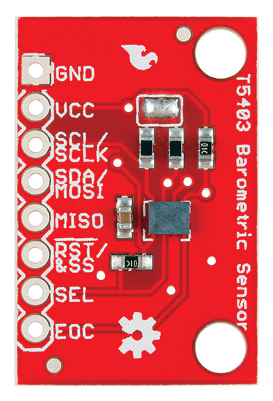
FIGURE 1. T5403 barometric pressure sensor with an I²C interface.

This sensor measures barometric pressure, turns it into an electrical signal, and then encodes this in an I²C digital interface.

All the electronics on the sensor board — the sensor itself, the analog front end, the ASIC, and the memory — dramatically simplify what we must do to integrate this sensor with the microcontroller. In this case, just plug it into a few digital pins and install the library. All the low level functions of reading the resistance, converting it to a voltage, filtering it, conditioning it, even compensating the electronics with the measured onboard temperature, and ending up with a calibrated barometric pressure is all done “under the hood” for us by the electronics shown in Figure 2. That’s a lot of processing power in a tiny space.

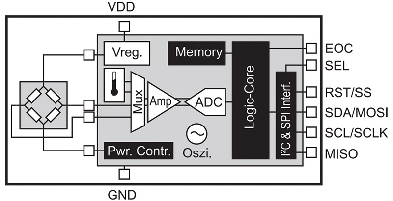
FIGURE 2. The electronics that turn the resistance measurement into an I²C signal that is then read by the microcontroller (source: EPCOS datasheet).

Some sensors output a low level digital signal, like a rain gauge. This sensor just sends a click every time a bucket is filled and emptied. It’s up to us to count the clicks with a digital I/O pin and keep track of the total rain fall.

Then, there are all the sensors which just output an analog signal. This is where the analog front end conditioning we add to the system can dramatically improve the quality of the measured information.

Limitations to Sensor Measurements in an Arduino

An example of a sensor which outputs a voltage is the TMP36 temperature sensor also from SparkFun. It comes in a small three-terminal plastic package shown in Figure 3.

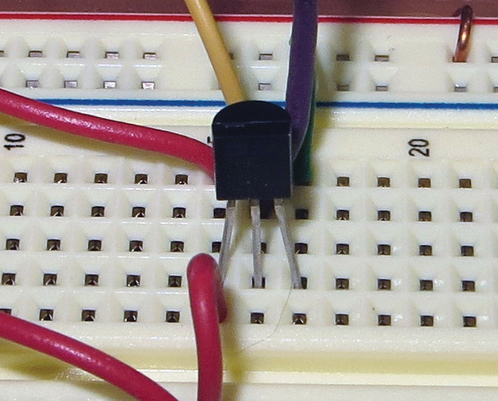
FIGURE 3. Close-up of the TMP36 temperature sensor.

One pin is connected to +5V; another pin is connected to gnd; and the middle pin is the voltage output that is directly proportional to temperature, with a sensitivity of 10 mV/°C and 0V at -50°C, or 100°C/V.

The output voltage from this temperature sensor can be read directly by one of the analog input pins on the Arduino. Here’s where we encounter the fundamental limitations with the Arduino analog input pins.

Each analog input pin of the Arduino is a 10-bit ADC (analog-to-digital converter). This means there are only 2^10 = 1024 discrete voltage levels the ADC can report. When we “read” an analog pin, the integer that comes back is a discrete level — a number between 0 and 1023. We sometimes refer to the units of these levels as analog-to-digital units (ADUs). When analog accuracy is important, or in general as a good habit, I use the 3.3V onboard reference as the reference to the ADC channels (see the sidebar). I also add a large capacitor to the reference channel just to reduce any AC noise on this rail.

With a voltage scale of 0V to 3.3V, this means the voltage resolution is 3.3/1023 = 3.2 mV resolution. In general, we should measure the reference voltage level for the ADC, Vref, with a three-digit DMM. Then, the voltage on the pin in volts is V[volts] = ADUs/1023*Vref.

The TMP36 sensitivity is 100°C/V. With a discrete level resolution of about 3.2 mV, the Arduino has about a 0.3°C per ADU resolution. This may be fine for reporting ambient temperature, but may not be sensitive enough when we care about very small temperature changes.

I wrote a sketch to read one of the analog channels of an Arduino Redboard from SparkFun. I averaged about 100 readings in about 100 msec, and scaled the voltage into a temperature value. The analog channel reading in ADUs was converted into a temperature in my sketch using temp [degC] = (ADU/1023 x Vref) * 100 – 50. The 50 is there because the output voltage is 0V at -50°C.

I printed the temperature values every 100 msec to the serial port and used MakerPlot to read the serial port and plot the temperature. I did no calibration at all of the sensor. Figure 4 shows the measured temperature when I touched the sensor and let go.

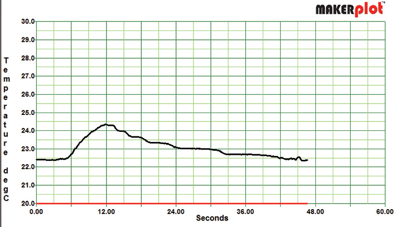
FIGURE 4. Measured temperature of the TMP36 when I touched it and let go.

In this example, you can see the ambient temperature of about 22°C before I touched the sensor. It rose about 2°C quickly in about three seconds. I let go and it cooled, taking a longer time.

On the cooling leg, you can clearly see the 0.3°C temperature steps corresponding to the resolution limit of the Arduino’s ADC. This is not a sensor limitation; it is an Arduino limitation.

When the signal we care about is a small signal, we just don’t have much sensitivity available from the 10-bit Arduino analog inputs.

Problem #1 is the small resolution available with the 10-bit ADC. We just can’t see small changes with only 3 mV resolution even using the smaller Vref of 3.3V.

Problem #2 is there is a DC offset on the signal (about 0.75V in this example). We can improve this by adding some gain, but we have to be careful not to exceed the 3.3V maximum voltage input to the ADC. This would be a maximum gain of about four.

Problem #3 — just marginally an issue with this sensor — is the output impedance of the sensor and what the ADC pin needs to see. Section 23.6.1 of the Atmel manual states: “The ADC is optimized for analog signals with an output impedance of approximately 10 kΩ or less.” Where this spec comes from is explained in the sidebar.

The output impedance of a sensor is a measure of how much current it can source or sink. According to its specs, the TMP36 has a maximum output current of about 50 uA of current draw possible. With roughly a 1V output voltage, this is an output impedance of 1 V/50 uA = 20K ohms. This is in the gray area of possibly a problem — especially when looking at fast data acquisition.

One way of getting around these three problems and enabling accurate and high resolution measurements from a wide variety of sensors is using an analog front end between the sensor output and the microcontroller input to condition the analog signal.

An Analog Front End Essential Element: the Op-Amp

We refer to all the electronics from the sensor element to the input pin of the ADC as the analog front end. While there is a huge variety of off-the-shelf building block circuits we can use in the analog front end, the two most important building blocks to solve all sensor interface problems are operational amplifiers and instrumentation amplifiers. An operational amplifier — affectionately shortened to op-amp — is a super high gain differential amplifier. Its output voltage is proportional to the difference in voltage between its two input pins, referred to as the V+ and V- inputs:

V_output = Gx (V₊ — V_-)

The value of G is often as high as 1,000,000. The secret to using op-amps effectively is using combinations of R and C elements in a feedback circuit to enable useful features. Whole books are written about op-amp circuits with specialized functions. A really great handbook by the legendary Walter Jung called Op-Amp Applications Handbook can be downloaded for free. The circuit we’ll look at in this article is the non-inverting amplifier.

In the non-inverting amplifier, the input signal goes into the V+ pin, and a simple resistor divider circuit connects the output pin to the V- input as shown in Figure 5.

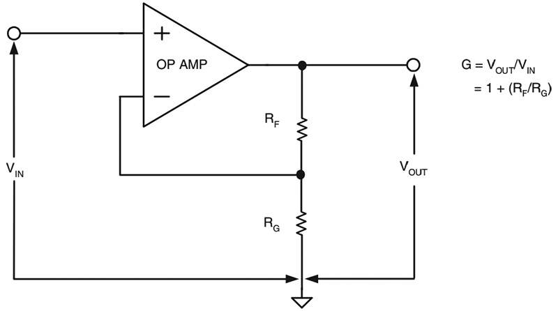
FIGURE 5. Circuit diagram of the non-inverting amplifiers using an op-amp, taken from Walter Jung’s Op-Amp Applications Handbook.

The gain in this circuit is:

Since this amplifier is often the first circuit to interface with a sensor, it is sometimes referred to as a pre-amp. An important feature of the amplifier — in addition to amplifying the signal — is to change the output impedance of the sensor. It can take a sensor with really high output impedance and provide a comparable signal level (or even higher) with an output impedance of a few ohms. This solves problem #3.

Among the three top suppliers of op-amps — Analog Devices, Linear Technology, and Texas Instruments (TI) — there are almost 500 different versions to choose from. I found one that I use all the time because it has pretty good specs, runs off the +5V single supply from an Arduino, and comes in an eight-pin DIP. Best of all, it only costs $0.29. As a bonus, it comes with two independent op-amps in one package for this low price.

I use the LM358 op-amp — manufactured by TI and available from Jameco and other distributors. It’s not the highest performance op-amp, but at this price, is a great general-purpose version and is incredibly easy to use.

In the application of the TMP36 temperature sensor, the nominal output signal level is about 0.75V at room temperature. I wanted to increase this signal level so it is higher, but still below the 3.3V of the Vref. I chose to use a gain of about three, resulting in a nominal voltage level out of the op-amp of about 2.25V. I used resistors of 22K ohms and 9.8K ohms, resulting in a gain factor of (1 + 22K/9.8K) = 3.245.

The original sensitivity of the TMP36 sensor was 100°C/V. With a resolution of 0.0032V, this is a temperature resolution of 0.32°C.

With a gain of 3.245, the output sensitivity of the pre-amp is 100/3.245 = 30.8°C/V. The voltage resolution of the 10-bit ADC is still 0.00323V, but this is now equivalent to 30.8 x 0.00323 = 0.1°C. Much better.

This helps solve problem #1. Figure 6 shows the recording of the raw output from the TMP36 sensor into A0 of the Arduino’s ADC, and the output of the LM358 with the gain of 3.245 into A1.

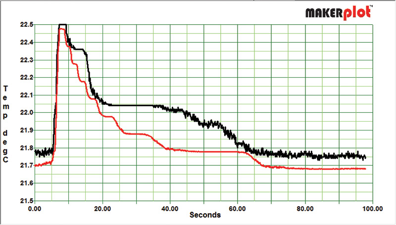
FIGURE 6. Measured temperatures of the same TMP36 using the scaled value directly from the sensor and after a gain of 3.245 in a pre-amp. Note the resolution improvement from 0.3° to 0.1°.

I converted the ADU values from A1 into temperature using:

Temp[degC] = (ADU/1023*Vref/Gain_opAmp) x 100 — 50

An Analog Front End Essential Element: the Instrumentation Amplifier

We still have problem #2. The voltage out of the pre-amp is about 2.5V. We want to see small changes on top of this large DC value. We really would like to subtract off a DC value and amplify what is left. This is the perfect job for an instrumentation amplifier.

An instrumentation amplifier is very similar to an op-amp. Its output voltage is related to the difference voltage between its two inputs by:

V_output = Gx (V₊ — V_-)

However, the gain in an instrumentation amplifier is typically adjustable from only 1 to 1,000. It does not use feedback from the output voltage to the input; instead it’s just a straight up differential amplifier.

Instrumentation amplifiers are most commonly used to amplify small differential signals such as in electrocardiogram monitoring or in resistance based sensors. They are at the heart of a Wheatstone bridge.

For our temperature sensor application, we can use the instrumentation amplifier to subtract off the DC voltage we provide at the V- pin and amplify what is left.

There are hundreds of different instrumentation amplifier options to choose from — each with slightly different specs and price points. The instrumentation amplifier I use the most with an Arduino is the AD623 manufactured by Analog Devices and available from Jameco.

It runs off the single +5V from the Arduino, comes in an eight-pin DIP package, is really easy to set up, and costs less than $5. The gain is selectable with a single resistor, Rg, from 1 to 1,000 using:

Rg = 100 kΩ/(G − 1)

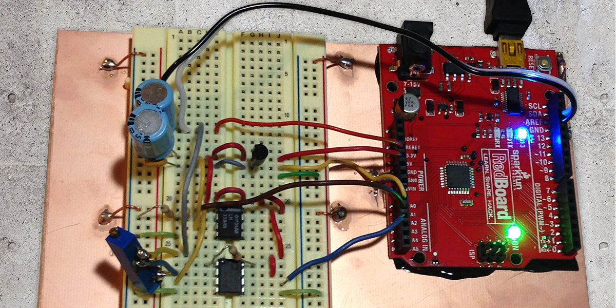
In this application, I wanted to use a gain of 10. The DC voltage was provided by a simple 10K ohm 10-turn pot connected between the 3.3V reference and ground. The center tap signal — which I could adjust — was connected to the V- input of the AD623. The final circuit with the TMP36, pre-amp, and instrumentation amplifier is shown in Figure 7.

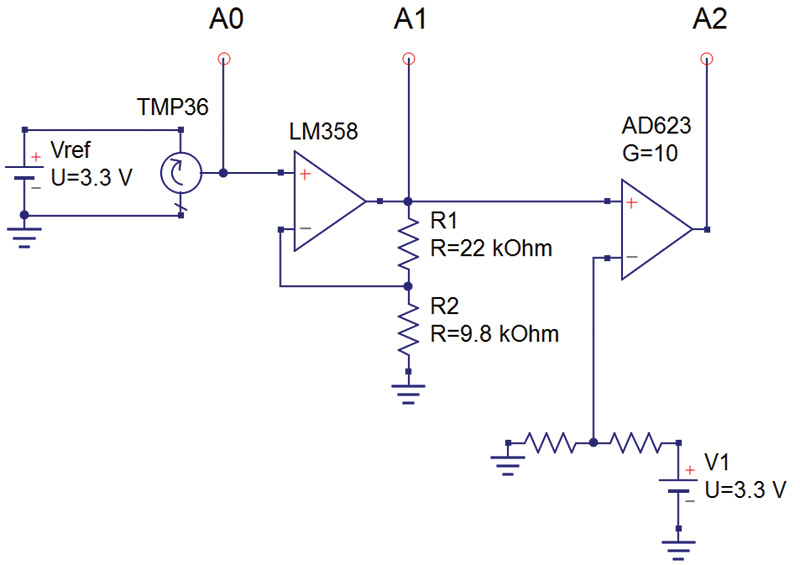
FIGURE 7. Complete circuit with sensor, pre-amp, and instrumentation amplifier.

This analog front end circuit was implemented in a breadboard adjacent to the Arduino Redboard. The amplifiers were powered off of the 5V rail of the Redboard. The two sensitive voltages used the 3.3V reference pin on the Redboard.

I added a few capacitors to the voltage rails to keep the noise down. Figure 8 shows this configuration.

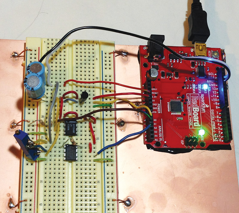
FIGURE 8. The complete system configured on a breadboard connected to an Arduino.

In this circuit, the original 100°C/V sensitivity was changed to 100°C/V /3.245/10 = 3.1°C/V. With a resolution of the least significant bit still 0.00323V, the temperature resolution is 3.1 x 0.00323 = 0.01°C. Now we’re talking.

We have three different sensitivity levels of temperature measured in this circuit: the direct readings; the direct readings increased in sensitivity by 3x; and the direct reading increased in sensitivity by 30x. All the conversion from ADUs into voltage and then into temperature is done in the sketch.

It’s the final temperature values which were printed to the serial port and available for plotting by my favorite plotting tool, MakerPlot.

With these three different temperature readings available, I did the same experiment: touching the sensor very briefly and watching the temperature rise quickly and fall slowly. In the slow decline in temperature, the resolution limits of 0.3°C and 0.1°C are clearly seen.

The smoothly varying temperature on this plotted scale of 0.1°C per division is an indication of the 0.01°C resolution of the signal after the instrumentation amplifier. Figure 9 shows these comparisons.

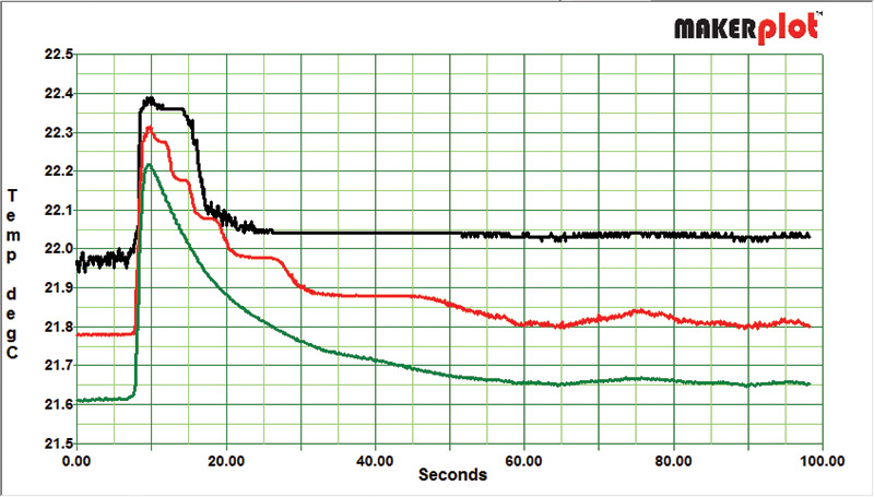
FIGURE 9. Shows the same experiment as before. I touched the sensor briefly and recorded the unconditioned voltage from the sensor, the voltage from the pre-amp, and the voltage from the instrumentation amplifier. You can see the impact of the higher sensitivity on the smoothness of the plots. Top trace: Resolution of 0.3°C from the TMP36. Middle trace: Resolution of 0.1°C from the pre-amp. Bottom trace: Resolution of 0.01°C from the instrumentation amplifier.

Conclusion

When we have the good fortune of using a sensor with a high level voltage and a low output impedance, we can just connect it to one of the ADC pins of an Arduino and get 10 bits of resolution with little effort.

However, if we want to push the limits of sensitivity or take advantage of sensors which have high output impedance, small scale signals, or small signals riding on a large DC offset, we can leverage an analog front end to condition the signal and get the most value from the 10-bit ADC in the Arduino.

Two essential devices dramatically simplify the design and implementation of an analog front end: the op-amp and the instrumentation amplifier. The LM358 op-amp is the perfect general-purpose version and the AD623 is the perfect general-purpose instrumentation amplifier which play well with an Arduino.

Of course, there is often more than one right answer to any design challenge and there are multiple ways of interfacing sensors to a microcontroller. The op-amp and instrumentation amplifier are sharp arrows to have in your quiver of design solutions.

To ensure the integrity of the measurements in this article, I incorporated a cat scanner to monitor each operation.

Figure 10 shows the bench set up with the cat scanner in operation. NV

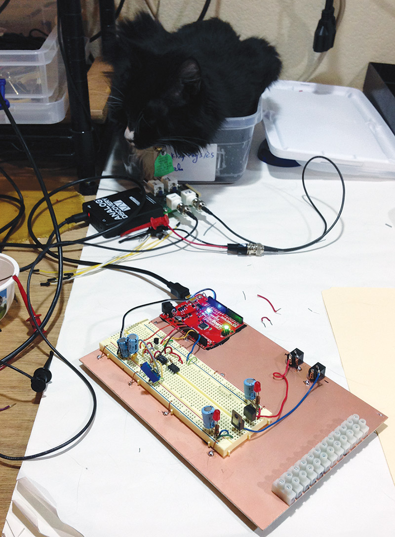
FIGURE 10. Maxwell — the cat scanner — monitoring every aspect of this experiment.

Improve the Quality of Your Analog Measurement Using the 3.3V Pin as the Vref

The ADC (analog-to-digital converter) pins of the Arduino compare the voltage at their input to a reference voltage to generate the 1024 different output levels. The default condition is to use the +5V rail on the die of the microcontroller as the reference voltage.

You might think that the + 5V rail is very low noise; after all, it comes from either the regulated USB power supply or the onboard regulated +5V supply if you are using an external power supply. If the microcontroller is not driving any outputs and its current draw on the power rail is low, then the noise on the power rail can, in fact, be low.

I wrote a sketch for my Arduino to toggle five digital outputs off and on really fast. The rail noise I measured on the board was about 5 mV peak-to-peak when the outputs were switching, but not driving anything. This is about the resolution of the ADC and would contribute negligible ADC measurement noise.

However, when the digital I/O pins draw some current, this has to come through the impedance of the power rail supply and its output voltage — which everything on-die uses — will drop.

I connected the five toggling outputs into 330 ohm resistors which then drove LEDs. We can estimate the current draw of each I/O. There is about 25 ohms of output impedance on the output transistor of each Arduino I/O pin. There is about a 2V drop across an LED. If the output voltage from one I/O pin when not driving a load is 5V, then the voltage drop across the (25 + 330) ohm resistors is 5V – 2V = 3V, and the current draw from the pin and the power rail per pin is:

I had five I/O pins toggling. This was a total current draw of 8.5 mA x 5 = 42 mA of current from the +5V rail. I measured the voltage drop on the +5V rail on the board as about 35 mV peak-to-peak. This corresponds to an output impedance of the power supply of:

This is very close to what I measured independently for a USB power supply. I measured an onboard regulator output impedance of the Redboard (when powered by an external 9V supply) to be 1.4 ohms, in comparison.

This 35 mV of noise on the board level power rail is almost identical to what I measured as the rail noise on the die itself. Of course, we can’t probe the on-die power rail directly, but we can see the on-die power rail voltage by setting a digital I/O pin as HIGH, and measuring its output voltage. After all, when its output is HIGH, the output pin is effectively connected to the +5V on-die voltage rail. This is the same voltage that would be used by the ADC reference channel in its default condition. Figure A shows all the measured voltages.

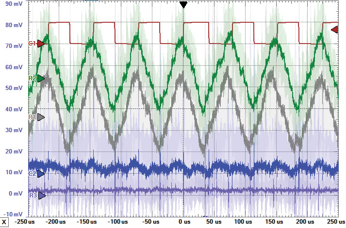
FIGURE A. Voltage noise on the various power rails while five digital I/Os toggled off and on. Top trace: Voltage on one of the digital pins showing its voltage switching. Next two traces down: Measured rail voltage noise on the board and on the output of a digital pin set to HIGH. This shows the 35 mV noise on the power rail when 42 mA of current switches. Fourth trace down: The +5 V rail voltage noise on the board with no current drawn by the I/O. The noise level is down to 5 mV. Bottom trace: Voltage noise on the +3.3 V reference with 42 mA of switching current. The scale for all except the digital I/O signal is 10 mV/div. The triangle shape is because the five I/O are sequentially turned on one at a time and then turned off one at a time.

The consequence of this is that when there is little current drawn by the microcontroller, there is probably no impact on the measurement accuracy of the ADC channels. However, if the microcontroller is also switching current around, the reference voltage will drop and this will contribute to measurement errors in the ADC values.

More importantly, this voltage noise on the Vref line will introduce errors; the magnitude of which will depend on what else the microcontroller is doing. This sort of problem is incredibly hard to debug. Better to avoid the chance of it ever happening.

The way around this problem is to use either another external reference voltage source or use the 3.3V reference supply brought out on many Arduino boards. On the SparkFun Redboard, this is a separately regulated supply which has nothing connected to it. Its voltage noise is very low. I measured it to be less than 2 mV peak-to-peak — even with 42 mA of switching current from the I/O pins.

Since it is available for free, it’s always a good habit to use this as the ADC Vref. The downside is that this will limit the maximum voltage range the ADC can sense. With an analog front end, this is not an important limitation.

To use an external reference voltage, in the void setup() function, you must add the line:

analogReference(EXTERNAL);

I also measure the analog reference voltage with a three-digit DMM and add a line near the beginning of each sketch where I can add the specific reference voltage level:

float Vref = 3.290;

Then, when I read an analog pin, I can calculate the actual voltage on that pin using:

Value_volts = analogRead(A0) /1023 * Vref

The Input Impedance of an Arduino ADC Pin

The Arduino input impedance of an ADC (analog-to-digital converter) pin is specified as 100 megohms. It sounds high and would be wonderful, but this is not the complete story. The first circuit element the pin sees on-die is a multiplexer which switches each of the six Arduino ADC pins into the actual sample and hold circuitry to be read by the ADC circuitry. This input has the equivalent of 14 pF of capacitance.

When the Arduino pin is read, the pin is switched into this capacitance. The sensor driving this pin must charge up this 14 pF of capacitance before it is read to get an accurate value. If it is still charging when the pin is read, the value will be inaccurate.

If the source impedance of the sensor is 10K ohms, then the RC time constant is 10^4 ohms x 14 x 10^-12 F = 0.14 usec. If we wait for six time constants, the signal will be within 0.2% of its final value. This is 1 µsec — about the fastest possible acquisition time for an analog channel.

If the output impedance of the sensor looks like a resistor of no more than 10K ohms, then the voltage read by the ADC will have settled to its final value before the voltage is actually read. If the output impedance is larger than 10K ohms, there is a chance the voltage will not have stabilized before it is read and the first measurement may not be accurate.

This sort of problem is incredibly hard to debug. As risk reduction in your design, just avoid the problem by always using a low enough output impedance for the sensor.

This is the origin of the Atmel spec recommending the sensor output impedance be less than 10K ohms to drive one of the ADC pins and not lose accuracy even in the worst case.