Turn your oscilloscope into a "Storm Scope" and detect lightning at distances up to 100 miles!
Lightning is a familiar and often feared natural phenomenon. Although lightning is seen in all areas of the country, southern Arizona and central Florida are areas of extremely high flash density (i.e., the number of cloud-to-ground strikes per square mile per year). When lightning strikes, property can be damaged, fires started, trees can be split in two (or, oddly, the bark can come off leaving the tree core intact), and, sadly, sometimes people are killed. It’s not surprising that the electrical power industry is a leader in lightning research because of the damage done to their power lines by lightning.
Human casualties are common. The daughter of a former governor of Virginia was struck at the National Guard Camp at Pendleton (Virginia) beach in southeast Virginia. Florida saw 298 confirmed lightning deaths in the 30-year period 1959 to 1989. Between 1940 and 1989, there were 8,103 confirmed lightning deaths in the United States (SIRS 1990, Earth Science, Article 67). According to the National Oceanic and Atmospheric Administration (NOAA), lightning killed 88 people in 1995.
About 30 percent of the people struck each year are killed. I would have guessed that nearly all of them would have been killed, with only a few survivors. But the statistics apparently suggest otherwise. Those people who are killed usually succumb to cardiac arrest. The survivors frequently suffer serious heart problems thereafter, and most have to be treated for severe burns. One source claimed that there are cases on record where lightning did not even break the skin, but traveled the wet surface of their body to ground. The skin was said to be severely burned, after the manner of scalding.
It is estimated that the earth is struck by lightning 20 million times per year. And if you believe the old myth about “lightning never strikes the same place twice,” then consider the fact that the Empire State Building in New York City takes about 12 strikes per year. Radio and television antenna towers are also struck frequently, although I hasten to add that they do not “attract” lightning that would not have come anyway (they tend to act as lightning rods).
The lightning is generated under up to 15,000,000 volts of electrical potential. According to one source, there is normally an atmospheric potential cloud-to-ground of 200,000 to 500,000 volts, and a constant but miniscule current of 10-12 amperes. The temperature inside the lightning bolt is 15,000 to 60,000 degrees Centigrade, which is several times the temperature on the sun. The lightning bolt travels at speeds up to 100,000,000 feet per second. A lightning bolt is actually a series of strokes, averaging about four. Durations vary from a few nanoseconds upward, but about 30 microseconds (30 µS) is said to be average. The average peak power per stroke is 1012 watts.
Most Common Activities Leading to Lightning Strikes on Humans
(according to NASA)
1. Working, playing, or walking in open fields.
2. Boating, fishing, swimming.
3. Working on heavy farm or road construction equipment.
4. Playing golf (!!!).
5. Talking on the telephone.
6. Using electrical appliances.
Many people struck by lightning were in unsafe situations. For example, on an open beach or in an open field such as a golf course. It is also not smart to be in a boat on the water. Standing next to a tree or other tall object (e.g., radio tower) is also rather dangerous, as the lightning may easily be attracted to that tree. In one case, a group of golfers in Massachusetts were struck when lightning struck a nearby tree, then traveled underground to a covered pavilion where they had taken refuge from the storm. Carrying an umbrella with a metal tip above the canopy has caused lightning injuries, presumably because it looks to the lightning like a lightning rod ... and you look like a ground wire!
As a general (but not absolute) rule, as long as you can hear thunder, the danger of strike is small. Lightning travels at the speed of light (3 x 10⁸ meters/second), while sound travels at 331.3 meters per second at 0°C (sound velocity changes a bit with air temperature), or 1,087 feet per second. As a result, the flash of light arrives instantaneously, while the sound of thunder arrives a short time later (measured in seconds).
A “rule of thumb” is to count the seconds between the flash and thunder clap, and then divide by five, to find the number of miles to the lightning bolt. One reason why I doubt validity of the “can hear thunder” advice is that I’ve been under thunderstorms where the lightning flash and thunder were very nearly simultaneous, indicating it was right overhead.
More precise measurements of distance can be done using a good stopwatch to measure the time of arrival of the thunderclap. From that data, you can calculate the distance from D = VT, where D is the distance and V is the velocity (if you use m/s for T, then D is in meters, but if ft/s is used, T is in feet). You can further refine your measurements by consulting a table of sound velocity related to temperature and atmospheric pressures.
Some Lightning Detection History
Before we talk about early lightning research, let me hasten to add a caution: DON’T EVEN THINK ABOUT DOING THESE EXPERIMENTS YOURSELF! People who’ve tried to duplicate these experiments have been killed in the attempt.
Electrical phenomenon was researched starting in the early eighteenth century. It was noticed that certain substances, when rubbed, produced static electricity arcs. It was also found that a type of capacitor called a Leyden Jar could store an electrical charge. It was believed — correctly, of course — that these sparks looked enough like lightning to suggest a connection.
In May 1752, Thomas Francois D’Alibard in France performed an experiment that Benjamin Franklin had failed at the year before. The experimenter stood on an electrical stand, holding an iron rod in one hand. The idea was to produce an electrical arc between that rod and another rod in the other hand connected to a grounded iron wire. In an attempt to repeat the experiment in July 1753, Swedish physicist G.W. Richmann, working in Russia, was killed by the lightning.
Benjamin Franklin conducted his famous kite experiment in 1752. He used a rain-damped kite string connected to a key at the bottom. The lightning traveled down the string, and jumped from the key to a dry silk ribbon tied to Franklin’s knuckles, and then through his grounded body. Others who attempted this experiment were killed. It’s interesting to wonder what the American republic would look like if Franklin, having been killed in 1752, was not alive to provide wisdom to the Constitutional Convention (his compromise suggestion, which reconciled the “large states vs. small states” controversy, is supposedly how we got the bicameral Congress).
When photography and spectroscopy were invented in the nineteenth century, additional facts were learned about lightning. Time-resolved photography was used to count the number of strokes per lightning strike. Current measurements were made by Pockels in Germany during 1897-1900. He analyzed the magnetic fields induced by the lightning currents to estimate the current level from basic electrical fundamentals. C.T.R. Wilson (ca. 1920s), who also invented the cloud chamber, used electric field measurements to study lightning. Wilson hypothesized that the electrical fields cause such great ionization, that it’s possible for discharges to occur between the clouds and the upper atmosphere. Seeming confirmation of the 1925 theory was provided on April 28, 1990 when Shuttle mission STS-32 videotaped a single luminous discharge in the stratosphere.
Modern lightning research still measures electrical and magnetic fields, but adds other techniques to their armamentarium. Cameras with electrically-triggered shutters can be used with photosensors to make photographs of lightning strikes. High-speed movie cameras are also used, although the invention of charge coupled device (CCD) sensors (which are used in video cameras) has allowed a number of new instruments to emerge.
Other researchers rely on radiowaves, especially the whistlers, spherics, and broadband RF noise generated in the ELF/VLF/LF portions of the radio spectrum. This type of research is also easily conducted by amateur scientists.
At a site in Florida, researchers fire three-foot high solid fuel rockets into thunderclouds. The rocket trails a grounded wire that conducts the stroke to earth (AMATEUR ROCKETEERS: DON’T DO THIS!). The Space Shuttle and satellites are also being used for lightning research. Some hauntingly beautiful video clips of space shuttle lightning are available from NASA web sites. High altitude aircraft lightning research revealed newly discovered phenomenon called sprites and jets.
Types of Lightning
Cloud-to-ground lightning passes from a cloud overhead to the earth beneath. Most cloud-to-ground strikes occur in the higher latitudes, although recent research indicates a more important variable is cloud top height. Cloud-to-ground ligthning is what causes injury and damages. Cloud-to-cloud or “inter-cloud” lightning passes from one cloud to another. Intra-cloud lightning appears within a single cloud. The “jagged” lightning that we see so often is called chain lightning, while sheet lightning is a generalized bright flash.
Other types of lightning may or may not be little more than myths, poor observations (e.g., optical illusions), variations on other types, or real, depending on who you consult. These include ball lightning, tubular lightning, bead lightning, silent lightning, cloud-to-air lightning (as opposed to cloud-to-cloud), and heat lightning.
Storm Scope
Lightning research can be terribly dangerous, especially if it puts you out in the open or if you are foolish enough to mimic professional methods such as ground wire tethered rockets. There are, however, some instruments that are easily built and relatively safe to use. The storm scope is one such instrument.
Figure 1 shows the basic configuration. This project was originally published by Thomas P. Leary in the June 1964 QST magazine (although his implementation used vacuum tube amplifiers).

FIGURE 1. Storm Scope Basic Configuration
The storm scope consists of a pair of orthogonal small loop antennas; one oriented North-South (N-S loop) and the other East-West (E-W loop). Keep in mind that a small loop antenna (e.g., < 0.18l wire length) shows a figure-8 pattern with nulls broadside to the loop plane, and maxima off the ends. Align the ends of the loop (maximum sensitivity direction) in E-W and N-S directions. A compass will make the accuracy better.
The loops are fed through differential amplifiers, with gains in the 20 to 80 dB range, to the vertical and horizontal plates of the oscilloscope. The reason for the wide gain scale is that oscilloscopes vary. The original project connected the amplifier outputs directly to the oscilloscope deflection plates. Modern two-channel oscilloscopes can be used in the X-Y to form a vectorscope, of which the storm scope is a variation on the theme.
Although any two-channel ’scope with an X-Y mode is usable, a directional ambiguity exists unless the ’scope also has a Z-axis (a.k.a., intensity modulation) input. This input is often present, but hidden on the rear panel of the ’scope. The Z-axis is used to intensity-modulate the screen with a signal from a sense whip or vertical antenna near the two-X loop. It may be necessary to amplify the Z-axis input signal, but in that case a single-ended rather than differential amplifier is used.
Figure 2 shows the loop and amplifier configuration. The loop consists of at least 50 turns (50-t.) of small gauge insulated wire in a three-foot (3-ft.) loop.
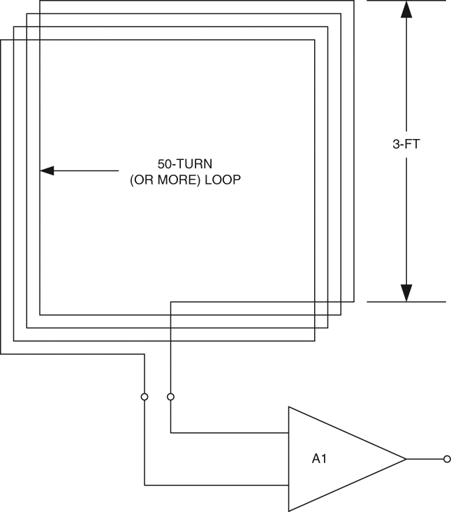
FIGURE 2. Loop & amplifier Configuration
Either square or circular loops can be used, although it appears to me that the square is more easily constructed. The loop is untuned. The output of the loop is applied to the input terminals of the differential or push-pull amplifier.
It is critical to shield the loops. Wrap either copper foil or aluminum foil (or tape) over the entire loop, except for a small quarter inch or so gap along the top edge (this prevents the shield from acting like a single-turn shorted loop itself). The shielded loop will be less prone to pattern distortions from capacitive coupling. In addition, it responds largely to the magnetic component of the lightning electromagnetic field. It is less sensitive to electrical fields, so will not pick up as much locally-generated power line and appliance noise.
I constructed a loop pair using 0.75” x 4” x 36” lumber. Although my own woodworking skills leave something to be desired (polite for “atrocious”), others are able to make a better job of the method shown in Figure 3.
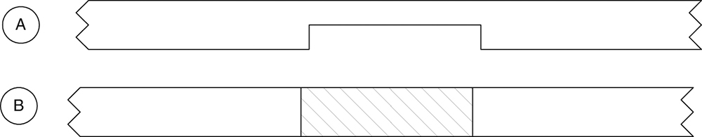
FIGURE 3.
A notch (Figure 3A) is cut at the center of the top and bottom members of each loop. The depth of the notch is the thickness of the lumber, while the width is sufficient to snug-fit the other piece of wood in it (Figure 3B).
The square loop will tend to “trapazoid” out of shape if left to its own devices. As a result, some or all of the methods of Figure 4 are used at the four corners of each loop.
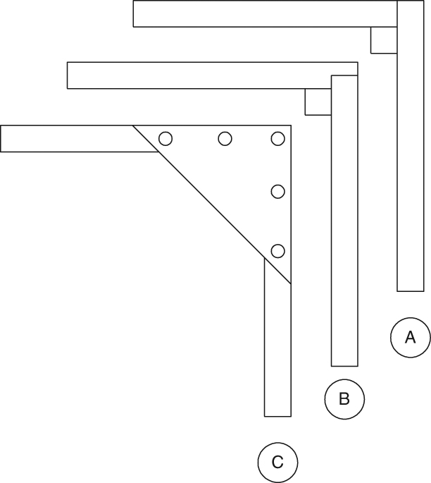
FIGURE 4.
In Figure 4A, the wood elements are butted together, glued, and nailed (or screw fastened). A small block, about 0.5 inch square and as wide as the loop arm, is glued in the corner to give strength. In Figure 4B, the same method is used, but the joint between the wood members is a bit different. I am told this method is stronger, even though it is more difficult. Finally, a triangular gusset plate cut from a thin sheet of plywood or spruce modeling lumber is shown in Figure 4C.
Figure 5 shows the wiring of the loop. I used 50 conductor ribbon cable, although one continuous loop of #26 (or so) enameled wire could be used as well (it takes more than 600 feet of wire per loop for this approach!).

FIGURE 5. Wiring of the loop
You can also use 60 or 64 conductor cable. The sensitivity of the loop is improved with more turns or a larger length per side. You can, for example, build a four-foot or five-foot loop, or use multiple runs of 50 conductor ribbon cable. In one case, a whistler/spheric hunter used 126 conductors made from intercom cable.
If you opt for the simpler ribbon cable method, then cross connect adjacent turns so that one continuous loop is formed. This is a tedious chore, but it’s made a lot easier if you use printed circuit perf-board (or some of the project boards from RadioShack) to make the connections. It is okay to lay the N-S and E-W loops over one another because their orthogonal geometry makes them minimally interactive.
Results to Expect
The original article claimed detection to distances of 500 miles, but I doubt that figure is practical. I would more likely guess tens of miles, or 100 miles, but further experimentation is needed to confirm the longer distance claim. Figure 6 shows typical patterns.
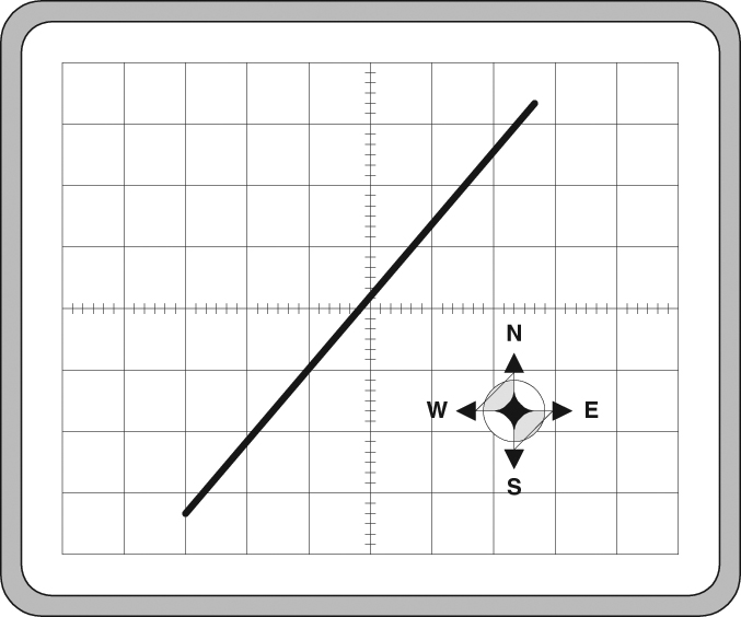
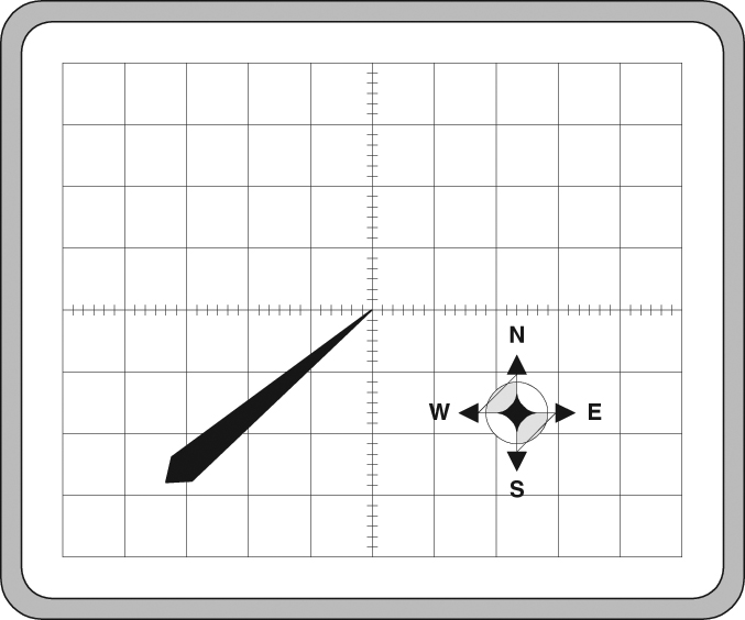
A - FIGURE 6 - B
These patterns are representations of what is observed, but are a bit more distinct and less ragged than actual ’scope photos (I am no longer able to photograph ’scope screens ... until I find a new hand-held Polaroid ’scope camera). I was able to create the patterns in Figures 6A and 6B, but those of Figures 6C and 6D are cribbed from the Leary article cited earlier.
The pattern in Figure 6A is what to expect when there is no Z-axis input to receive the vertical sense antenna signal. It shows the line of the storm, but has the directional ambiguity found on loop antennas. In other words, the storm could be in either direction from the loop. Figure 6B shows the pattern to expect when the sense antenna is used, and the Z-axis intensity is correctly adjusted. This is essentially the same concept as a sense antenna producing a cardioid pattern on a radio direction finding (RDF) antenna. The actual pattern will be a lot more ragged than shown here.
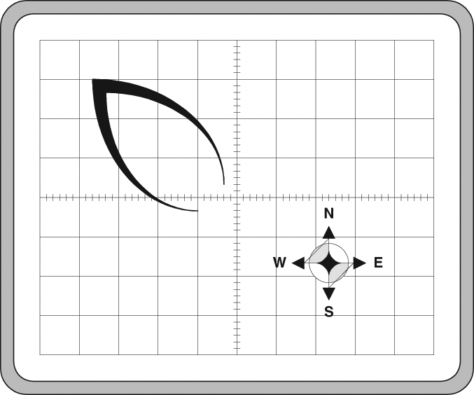
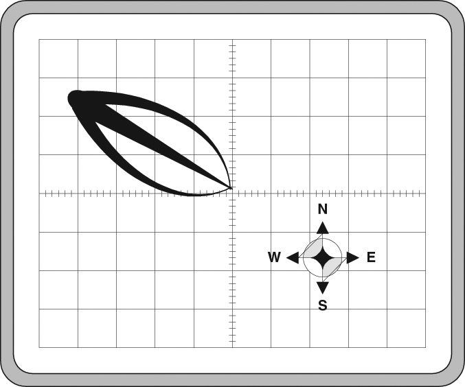
C - FIGURE 6 - D
Leary claims that patterns like Figure 6C are produced with horizontally polarized cloud-to-cloud discharges (the others were essentially groundwave signals). The pattern in Figure 6D represents what might be seen when a groundwave and cloud-to-cloud pattern co-exist. I was not able to confirm these patterns, but that might be the particular thunderstorm I observed when I was active in building loops while researching a book (Joe Carr’s Loop Antenna Handbook, Universal Radio Research, Reynoldsburg, OH). NV