The Smith Chart is one of the most useful tools in radio communications, but it is often misunderstood. The purpose of this article is to introduce you to the basics of the Smith Chart. After reading this, you will have a better understanding of impedance matching and VSWR — common parameters in a radio station.
The Inventor
The Smith Chart was invented by Phillip Smith, who was born in Lexington, MA on April 29, 1905. Smith attended Tufts College and was an active amateur radio operator with the callsign 1ANB. In 1928, he joined Bell Labs, where he became involved in the design of antennas for commercial AM broadcasting. Although Smith did a great deal of work with antennas, his expertise and passion focused on transmission lines. He relished the problem of matching the transmission line to the antenna; a component he considered matched the line to space.1
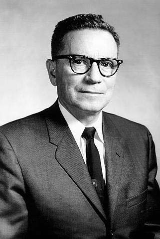
Phillip Smith — Inventor of the Smith Chart.
Smith developed the first graphical solution in the form of a rectangular plot from his measurements of the maxima and minima voltages along the transmission line. He used a thermocouple bridge and voltmeter to make the measurements. The first graphical chart was limited by the range of data so he came up with a polar plot that was a scaled version of the first plot. According to his biography, his impedance coordinates were not orthogonal — which means perpendicular — and there were no true circles, but the standing wave ratio was linear. This chart closely resembles the chart we see today.
What Is a Smith Chart?
Although there are many computer programs2, 3 and network analyzers that can solve impedance matching problems for you, a complete understanding of the Smith Chart is highly beneficial in understanding the nature of transmission lines. There is some algebra involved in understanding the basic transmission line equations, but — once you understand how to move on the graph — you can forget the math and just read the chart.
The Smith Chart is a polar plot of the complex reflection coefficient, Γ, for a normalized complex load impedance Zn = R + jX, where R is the resistance and X the reactance. A Smith Chart is utilized by examining the load and where the impedance must be matched. Sometimes, instead of considering the load impedance directly, you express its reflection coefficient, ΓL.
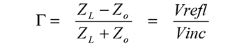
We know the reflection coefficient ΓL is defined as the ratio between the reflected voltage wave and the incident voltage wave, as shown in Figure 1.

Figure 1. Impedance at the load.
The reflection coefficient ΓL is related to the load impedance ZL and the system impedance Zo as:
There are resistance circles from 0 to “∞” Ohms. The reactance curves on the top half of the chart are inductance curves; most notable are the 0.9 and 1.0 curves at the top that curve down to the right hand center. Polar means there is a real part — the magnitude of the impedance point (or ΓL ) and the phase of the impedance. On the Smith Chart, the phase is actually the distance in wavelengths along the transmission line — the outer-most circle. Once you plot the impedance point, other parameters — like Voltage Standing Wave Ratio (VSWR) or return loss — can be read off the Smith Chart.
The center of the chart (r = 1.0 and x = 0) is always a “perfect match,” at least for a desired 50 Ohm, but can be any impedance you want. For the common 50 Ohm system, the center of the chart would be “normalized” to 1.0 units. All impedances are scaled relative to whatever characteristic impedance value you are working with.
VSWR can be depicted as a circle centered around the chart center (at “1.0”). One revolution around the VSWR circle is a one-half wavelength. The reason once around is only half a wavelength is due to the addition of two waves — the forward and reflective waves on the transmission line. For example, your transmitter sends a forward signal (Vinc) and some of this signal is reflected back from the load as Vrefl. Hence, the notion of “standing waves” comes from these two voltages. The smaller the SWR circle, the lower the return loss, and the better the impedance match. Understanding this principle proves that VSWR is constant along the transmission line. However, the resistive and reactive ratios do change along a line. Line loss increases VSWR by increasing the resistive component. This, too, is covered by the chart; read off the values by transcribing a line down to the scales at the bottom in decibels (dB) or voltage.
There are at least four other important points on the Smith Chart. Two of them represent an “open”: far right, where the resistive component is infinity, as well as a short and far left, where the resistive component is zero. The other two key points are at the extreme top and bottom points. At the top, you can see a “1.0,” which represents an impedance of +j*1.0, a pure inductor. At the bottom, you can also see a “1.0,” which represents an impedance of -j*1.0, a pure capacitor.
Every point in between represents the various combinations resulting from a mismatched condition and shows how far you are from the desired impedance — usually the center — and how to form the conjugate matching circuit. Simply plot the impedance of a load, then traverse the correct curves to reach the center (50 Ohms). This is easier said than done, so here’s an example that concerns an antenna with an input impedance of 50 –j40 Ohms, a 50 Ohm transmission line, and a transmitter with a desired output impedance of 50 + j0 Ohms.
A plot of the antenna load impedance is shown in Figure 2.
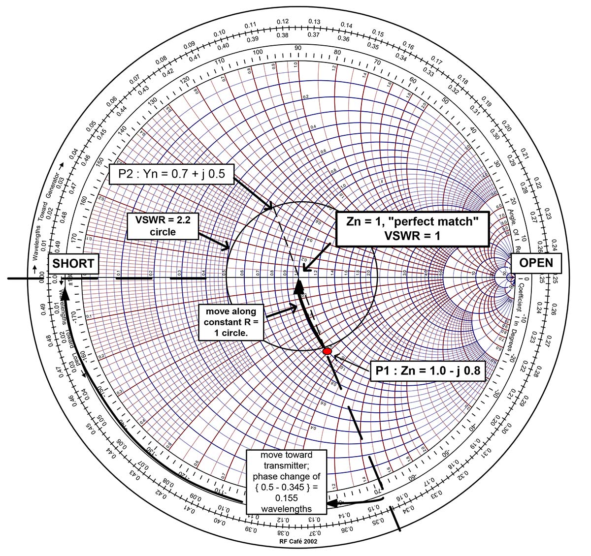
Figure 2. Smith Chart showing antenna load impedance “P1,” admittance point “P2,” and path “P1-to-center” for a series inductor to obtain a “perfect match” at the center point.
The normalized load impedance is 1.0 - j0.8. The desired, normalized impedance is then 1.0 – j0.8 + j0.8 = 1.0. Using a compass, you can draw a circle centered on 1.0 with the radius extending to the point “P1.” From the real axis and the intersection of this circle, draw a vertical tangent line to the SWR scale at the bottom of the chart. In this case, the SWR is approximately 2.2.
The following is a very important procedure in using the Impedance Chart. Movement along constant resistance circles in the clockwise direction means that you are adding series inductance. Movement along constant resistance circles in the counter-clockwise direction means that you are adding series capacitance. In this example, we can reach the center point — a perfect match — by adding a series inductor. How do we determine the inductance value?
The equation for inductive reactance is XL = 2 * π * F * L, where F is the frequency of operation. In the case of 21 MHz, XL = 2 * π * 21x106 * L * 50 = 0.8 and, by rearranging terms, we arrive at L = 0.12 nH.
It is important to point out that the Impedance Chart can be used with admittance points. The point “P2” in Figure 1 represents the load admittance of 0.7+ j0.5. It is obtained by traversing the SWR = 2.2 circle one-half revolution and drawing a line bisecting the circle. You can move from P2 to the other points, as well, but you will be adding shunt elements rather than series elements in your matching circuit.
Impedance and admittance curves are used interchangeably when dealing with series and shunt circuit elements. The contours of constant resistance and reactance can now be interpreted as normalized conductance G and susceptance, S. In an Admittance Chart, movement along constant conductance circles in the clockwise direction means that you are adding shunt capacitance. Movement along constant resistance circles in the counter-clockwise direction means that you are adding shunt inductance.
Conclusion
The advantage of the Smith Chart is that it can solve transmission line problems very quickly; also, it forces you to understand how to match a load to the transmitter. If you practice using the Smith Chart to solve antenna or transmission line matching issues, you will be comfortable with all sorts of related problems. The Smith Chart can be applied to other RF devices, including tank circuits, filters, transistors, microstrips, and other microwave elements where a specific parameter — like impedance, power, or line loss — is needed for the RF system. NV
References
- “Phillip H. Smith: A Brief Biography by Randy Rhea , Noble Publishing
- The ARRL Radio Designer also has a Smith Chart utility.
- Smith Chart computer program written by The Berne Institute of Engineering. A demo version can be obtained at http://sss-mag.com/zip/smith_v191.zip.