Editor's Note - This article discusses the use of SwitcherCAD/LTSpice as it was when the article was written. Links and some references have been updated, however the general content has not been updated to reflect any changes to the software in its current form. The current version of SwitcherCAD/LTSpice is now called LTSpice IV, from Linear Technology.
There is an old saying: Tell me something and I forget; show me something and I remember; let me do something and I learn. This is very true of electronics for most people. You can read books until you are blue in the face and in six months, you'll be lucky to remember where you left the book. Demonstrations of real hardware are more effective. And nearly everyone learns better in the lab with a handful of parts.
Paradoxically, when you need to learn the most, you probably have less lab equipment, parts, and tools, than someone who has more experience. But no matter what your experience level, it just isn't always practical to build a circuit just to experiment with it.
Luckily, with a PC, you can simulate nearly any circuit you can imagine with better results than you might expect. The secret is in a software program known as SPICE. SPICE has long been a tool for professionals with access to big computers. However, with powerful desktop PCs and some free or low-cost software, you can simulate nearly any circuit before you actually build it. In the process, you can develop a lot of real-world intuition about how circuits work without having to heat up that soldering iron.
Free Spice
The first thing to do is get a copy of SPICE. SPICE originates at Berkeley, and is free to distribute. However, the plain Berkeley version isn't very friendly to use. You enter circuits using a special text file and the program reports its results as a table of numbers or a crude ASCII plot. However, there are several Windows versions that can simplify using SPICE.
One of the best is absolutely free from Linear Technology Corporation and is known as LTSpice IV (Formerly known as SwitcherCAD). Linear offers this program to help you design switching power supplies using their products, but the program is really a very nice SPICE port with schematic capture and plotting functions built into it. What a great service for the electronics community and the fact that you'll think of them every time you use it seems fair enough. You can download the program at www.linear.com/designtools/software/.
SPICE uses models that represent different types of electronic components. SwitcherCAD III/LTSpice has quite a few models, but you can also add other models (often available from the component's manufacturer). The program can also handle digital simulation. If you prefer a more traditional SPICE, you might check out WinSPICE (www.winspice.co.uk/index.html). You can also find a list of inexpensive or free SPICE programs at www.terrypin.dial.pipex.com/ECADList.html.
If you use WinSPICE or another text-based SPICE, you might want to investigate a schematic drawing program that can automatically generate SPICE net lists (the text file that describes a SPICE schematic). Many schematic drawing programs can do this. For example, the popular Eagle (www.cadsoftusa.com) has an add-on user program that can export a SPICE net list (you have to download the add-on separately from their download page). In this article, I'll show you how to get started with SwitcherCAD III/LTSpice and I'll also show you a little about the more traditional usage of SPICE. In particular, I want to show you how you can gain intuition about circuits using your PC instead of a breadboard.
Getting Started
I'll assume you have SwitcherCAD/LTSpice installed. Start the program and use the File | New Schematic menu option. Draw the schematic shown in Figure 1.
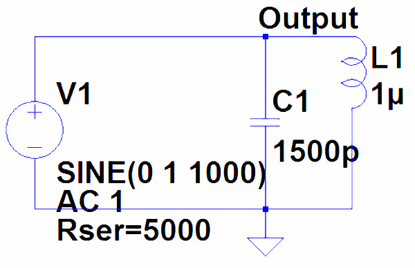
FIGURE 1.
First, use the toolbar icon that looks like an AND gate to drop a voltage, capacitor, and inductor component on the schematic. Then use the wire tool (looks like a pencil drawing a wire) to connect them together. Use the ground icon on the toolbar to include the ground and connect it too. Once all the wiring is connected, you can right click on each component to set its properties. For the capacitor, set the value to 1500p (1500 picofarads). For the inductor, set the value to 1u. This is a common way to specify SPICE values (see Table 1).
| Suffix |
Multiplier |
Common prefix |
| T |
1e12 |
Terra |
| G |
1e9 |
Giga |
| Meg |
1e6 |
Mega |
| K |
1e3 |
Kilo |
| mil |
25.4e-6 |
|
| m |
1e-3 |
Milli |
| u (or µ) |
1e-6 |
Micro |
| n |
1e-9 |
Nano |
| p |
1e-12 |
Pico |
| f |
1e-15 |
Femento |
TABLE 1. Suffixes recognized by SPICE
It is easy to forget that a 10M resistor is 10 milliohms not 10 megaohms (which would be 10Meg). For the voltage source, you'll need to right click and then click on the Advanced button. Select the sine voltage source and set the amplitude to 1 and the frequency to 1000. Also set the AC amplitude to 1 and the series resistance equal to 5000 (or 5k).
The next step is optional, but makes life a little easier. Use the toolbar button that looks like a letter A in a box. Type "Output" in the dialog box and then click on the wire going to the hot side of L1. This will label that wire as "Output" and you can refer to it as such in future work. If you don't do this, you have to use an internally-generated designator that the schematic drawing program arbitrarily selects.
Over Analysis
SPICE can perform many types of analysis. When you use the Simulate | Run menu, you'll get several choices:
- Linear AC Analysis — Sweeps an AC source and shows the resulting response.
- DC Sweep Analysis — Sweeps a DC source and shows the resulting response.
- Noise Analysis — Computes Johnson and Flicker noise.
- DC Operating Point Analysis — Computes the DC bias point (assumes capacitors are open and inductors are shorts).
- Non-Linear Transient Analysis — Provides an oscilloscope trace of the circuit as it operates.
- Small Signal DC Transfer Function Analysis — Computes the gain of the circuit.
For this example, pick Linear AC Analysis. The dialog box shows you that this is the SPICE .ac command and it also shows placeholders for the arguments the .ac command expects. You want to enter:
.ac lin 1024 1Meg 20Meg
This tells SPICE to sweep the AC voltage source from 1MHz to 20MHz in 1024 linear steps. The program places a special comment field on the schematic so you won't enter this again. After the analysis, you can right click on the comment to change the parameters. You can also delete it or use the .op toolbar button to insert a different command.
Once you enter the command, the program will prompt you for what you want to view. Pick V(output). This corresponds to the wire you labeled while drawing the schematic. You can also select different options. For this example, select Plot Magnitude and Magnitude Decibel and Frequency Logarithmic. Leave the other options unchecked. Figure 2 shows the results.
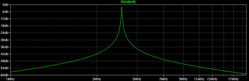
FIGURE 2.
You can click on a wire to see the voltage through that wire. Clicking on a component shows the current through that component. Since this is a parallel LC circuit, V(output) has a large spike at the resonant frequency. Away from that frequency, the network exhibits a good deal of loss rather quickly. If only that were true!
In real life, the sharpness of this spike de-pends on the circuit's Q. The Q depends on the internal resistance of the components and their reactance.
Capacitors typically have very high Qs, so let's focus on the inductor. Right now, the inductor is perfect. But in real life, we can't find perfect inductors. So right click on the inductor and set the series resistance to 0.5 Then run the simulation again (see Figure 2).
Notice the spike is not as sharp. Repeat the exercise with a series resistance of 5. The spike gets even broader. You can experiment with other effects (such as the capacitance inherent in the inductor). In particular, set the capacitor's series inductance to 1n and change the SPICE command to:
.ac lin 1024 1Meg 200Meg
Now when you run the simulation, you'll see a self-resonant notch above 100MHz and a slight effect on the spike (see Figure 3).
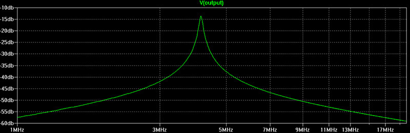
FIGURE 3.
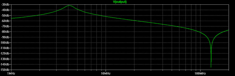
FiGURE 4.
That Was Too Easy!
If you prefer to use SPICE the old-fashioned way, you can do that too. Here is the net list for the circuit:
* D:\SwCADIII\lcpar.asc
V1 Output 0 SINE(0 1 1000) AC 1 Rser=5000
C1 Output 0 1500p
L1 Output 0 1<B5> Rser=5
.AC lin 1024 1Meg 200Meg
.end
The first line is simply a comment. The V1 line tells SPICE that there is a voltage source from node Output to node 0 (which is always ground). The C1 line shows a capacitor and the L1 line shows an inductor. The .AC command is the same as the one you plugged into the schematic editor. Of course, .end finishes the file.
Although it is tedious to make a circuit like this, many SPICE books and tutorials will use this format so it pays to know about it. Also, if you use a different SPICE, you may have to use this net list format (or use a schematic program to generate them automatically). LTSpice can process these files directly if you don't want to use the schematic editor.
A Switch
Next, try entering the circuit in Figure 5.
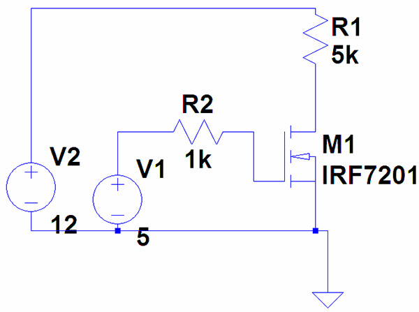
FIGURE 5.
The FET is a NMOS FET. You can right click on it to choose the exact type (an IRF7201, in this case). Place the output label on the drain of the FET (the terminal connected to R1).
In this circuit, V1 represents the output from a logic gate (perhaps the output pin of a BASIC Stamp). To see what would happen, you need to perform a DC sweep analysis. In particular:
.dc v1 0 5 .1
This tells SPICE to sweep V1 from 0 to 5 volts in .1 volt steps. The output of the analysis appears in Figure 6.
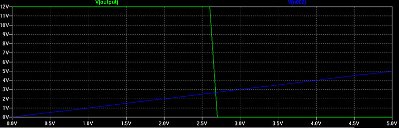
FIGURE 6.
Notice that around 2.7V, the FET switches on hard and the output voltage falls to about 0 volts.
If you want to see a "real world" simulation, right click on V1 and select Pulse. You'll enter the following parameters:
VInitial = 0
VOn = 5
TDelay = .5
TRise = 1n
TFall = 1n
TOn = .1
This creates a 100mS pulse. Now run a .TRAN simulation with an argument of 1 (this runs the circuit for one second). You can see an excerpt of the simulation's output in Figure 7.
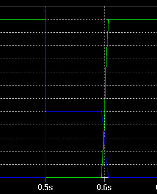
FIGURE 7.
You can see the effects of gate capacitance and switching times very clearly. This type of simulation is the closest to an ordinary oscilloscope display. You can even ask for an FFT of the data using the View | FFT command.
More About Spice
There are a few things that may not be obvious about using SPICE. For example, if you want to leave a node "hanging," just connect a current source with a 0 current between the node and ground. Similarly, if you want to measure a current in a path, you can put a 0V voltage source in the path which will allow you to measure the current.
Be sure to check out the help file to learn more about SPICE. You can download more models from many places on the web (for example, look at www.intusoft.com/slinks.htm). You can do many sophisticated analysis and modeling jobs with SPICE. But for all of its complexities, it is easy enough to use to model simple circuits. NV