Why is the sky blue? Why do birds sing? Why do I have 10 fingers? We all asked these questions when we were children. When I started to learn about control systems, I felt just like a kid again. I asked all sorts of questions. Why does a system overshoot? Why can’t I turn the gain up higher? Why is this system oscillating? It’s wonderful to be like a child again. There is so much to be learned.
In Part 1, we layed the foundation for the Proportional Integral Derivative PID controller. Using a simple, intuitive approach, we explored what each term represents. We examined how simple op-amp circuits could be used to construct the individual elements. In Part 2, we will see a complete analog PID system. We will explore the dynamic operation of the PID control system. We will explore how to operate and tune a PID controller. Using our servo motor example, we will explore system stability. We will learn new terms, such as overshoot, dampening, and oscillation. We will see how the individual P, I, and D terms come together to form a complete control system.
Last month, we came to several conclusions about each of the P, I, and D terms. These concepts are very important to our present discussion, so we will review them again. You can follow along with the block diagram shown in Figure 1.
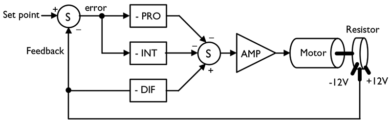
FIGURE 1. Block diagram of the DIP controller and servo motor.
Proportional Concepts (PRO)
A system will try to correct the error between the set point and the measured output. It does this by commanding the system in a direction that opposes the error. The intensity of the correction is determined by proportional gain. The proportional component provides a correction only if there is an error!
Integral Concepts (INT)
The integral section operates when an error is present. It accumulates this error over time. Therefore, a small error can become a large correction, given enough time. As the error is accumulated, the system will be forced to correct the error. Finally, the integrator will overshoot the set point. An error opposite of the original is required to discharge the capacitor.
Derivative Concepts (DIF)
The output of the differentiator is proportional to the speed of the system. If the system is moving fast, the output is high and vice versa. If the motor is not moving, the differential output will be zero. The differential term is applied in such a way as to slow down the motor.
Circuitry
A simplified schematic for the PID controller was printed in Part 1. A new, more advanced, schematic is presented here as Schematic 1.
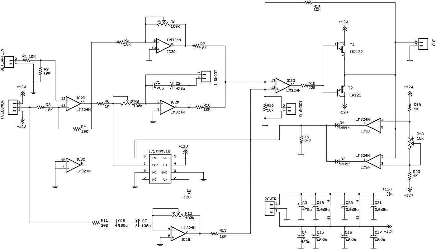
SCHEMATIC 1. The advanced PID controller schematic.
A new circuit has been added consisting of IC3A, IC3B, and IC1. Again, this circuit is an adaptation of the PID controller presented by Professor Jacob in his book, Industrial Control Electronics.
This new circuit is designed to prevent the integrator circuit from functioning under certain conditions. The reasons for this added feature will be explained later in this article. The analog switch (Maxim MAX318) disables the integrator by shorting the integrator’s input to ground. The analog switch is driven by op-amps IC3A and IC3B. This pair of op-amps forms what is commonly called a window detector. The name refers to the “window” of voltage where the op-amps have a low output (allow the integrator to function). If the output of the PID controller is above or below a certain point, the op-amps will turn on the analog switch, thereby disabling the integrator.
Construction
The circuit board shown in Photo 1 was designed for this article. You can download the cad files (Eagle) from the downloads section at the end of this article.
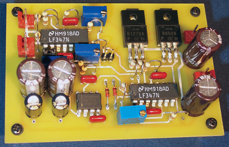
PHOTO 1. Complete analog PID controller.
The cad file is slightly different than the board shown here. I made a few minor modifications/improvements to the board. Feel free to use the CAD files as you see fit. In case you were wondering, Advanced Circuits manufactured this board. I am very happy with their service. Check out their website at www.4pcb.com — look for their bare bones special.
As an alternative to the PCB, you could construct the circuit using “dead bug” or perfboard construction. The layout isn’t critical. I was able to breadboard this circuit successfully. Just remember to keep the wire runs short and decouple the op-amps.
What Are We Controlling?
We will be controlling the position of a servo motor. Our servo motor is a mechanical device
Yes, this is an obvious statement, but take a moment to think about the attributes of a mechanical system. The moving parts of a motor have mass. Consequently, they have inertia and momentum. It takes a finite amount of time before the motor will respond. It takes time and energy to get the motor armature, gears, and load moving. Figure 2 shows how the modified HiTec HS-322 R/C servo motor responds when a 6 VDC signal is applied.
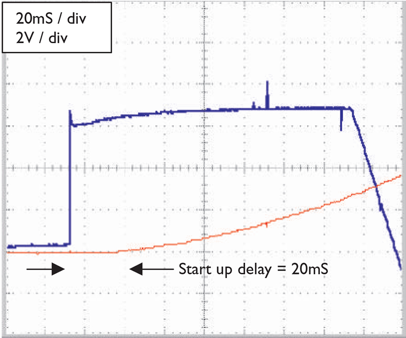
FIGURE 2. Delayed response of a modified HiTec HS-322 servo: blue = voltage applied to motor; red = motor response as measured via resistor.
We see that it takes approximately 20 mS before the motor even starts to move. Conversely, once the motor is moving, it does not want to slow down.
The motor is also an electrical device — again an obvious statement. The motor windings have the characteristics of an inductor and a resistor. Recall that an inductor works to keep the current constant. Consequently, when the motor is turned off, there is no current flow. When the voltage is first applied, the inductance of the windings tries to keep the current at zero. Therefore, the motor inductance accounts for some of the delay seen in Figure 2. The motor resistance also limits the amount of current and, thus, the torque that the motor can deliver.
How Do I Connect the Servo Motor?
In a word, carefully! Things can get out of control when designing and experimenting with control systems. In preparing this article, I stripped no less than three sets of gears out of the servo motors! After that, I got smart and added limit switches to the servo. Also, it is a good idea to put a current-limiting resistor in series with the motor — 10 to 20 ohms works nicely.
The PID loop requires negative feedback. If either the motor or feedback resistor is installed incorrectly, we will have positive feedback and the system will go nuts. Remember those limit switches!
When we first connect the PID, it is best to disable the integrator and differentiator. The integrator is disabled by shorting out the feedback capacitor. The differentiator is disabled by shorting out the resistor connected between IC3D and ground. These components are marked on Schematic 1. On my circuit board, I have added headers to facilitate this process. Just add a shunt on top of the headers to disable the integrator’s derivative section.
The motor and feedback resistor should be connected to the circuit. If possible, do not physically connect the motor shaft to the feedback resistor. If you are using a servo, the top may be opened and the final gear removed. Short the set point, i.e., 0 volts input. Apply power to the system. The motor will most likely turn. Move the feedback resistor. You should be able to make the motor change directions. The motor should turn in a direction opposite that of the feedback resistor. If it doesn’t, reverse the polarity of the motor.
At this point, we can physically connect the motor and the feedback resistor. Be ready to disconnect the power. Things can get out of hand quickly. When power is applied, the motor will either move the feedback resistor to midrange or the system will oscillate back and forth. If the system oscillates, decrease the proportional gain.
How Do I Tune a PID Controller?
This question is a bit like asking how to ride a bike. The best answer is to just do it. I chose the servo motor example as the basis of this article because it operates at just the right speed. The system is slow enough so that we can see what is happening, but not so slow that we have to wait to see our changes. This is nice because we can quickly tune the system. Taking this analogy further — tuning a PID controller is like riding a bicycle. We are trying to balance three criteria, as shown in Figure 3. An ideal system would be unconditionally stable. It would respond instantaneously to an input and it would have no error, i.e., it would go exactly where we tell it to.
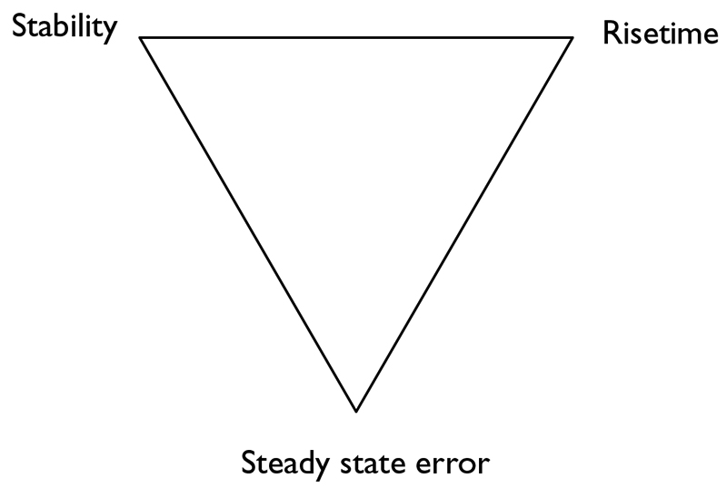
FIGURE 3. Factors to consider when tuning a control system. In general, you can optimize two, but not all three.
There is no such thing as an ideal system and our servo motor is no exception. We already know that the servo motor is a slow device. It takes over 20 mS before the motor starts moving. We also know that it will not stop instantaneously. Once it is moving, the momentum will keep it moving.
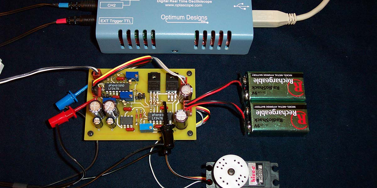
In real systems, we are left with compromises. We are left to balance stability, rise time, and steady state error. Let me explain using a series of oscilloscope views. The test set-up used to capture the “oscillographs” is shown in Photo 2. In the following sections, we will observe the “step response” of the servo motor system.
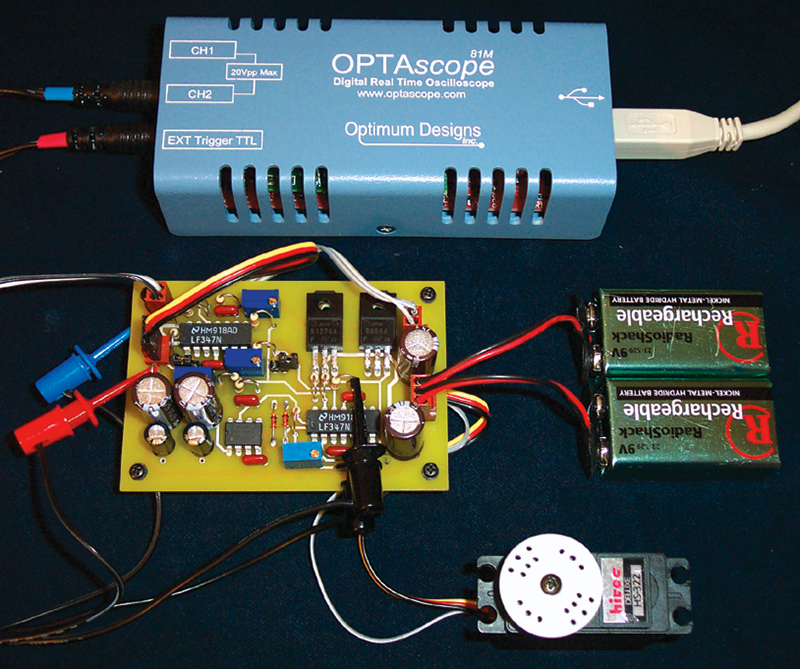
PHOTO 2. Test set-up for PID control of servo motor.
A step input is nothing more than a square wave. We are telling the servo motor to instantly move from one position to another. The blue line represents the step function applied to the input. The red line represents the actual response of the servo mechanism, as measured at the feedback resistor.
Proportional Control
We will first examine how the servo motor responds to changes in proportional gain. The integrator and differentiator should be disabled at this time. When we adjust the proportional gain, we are adjusting how hard the system will be driven. Higher proportional gains send more current to the motor. The motor will develop more torque and, as a result, will move faster. This results in a more responsive system that is better able to follow the set point. However, there is a limit, as can be seen in Figure 4.
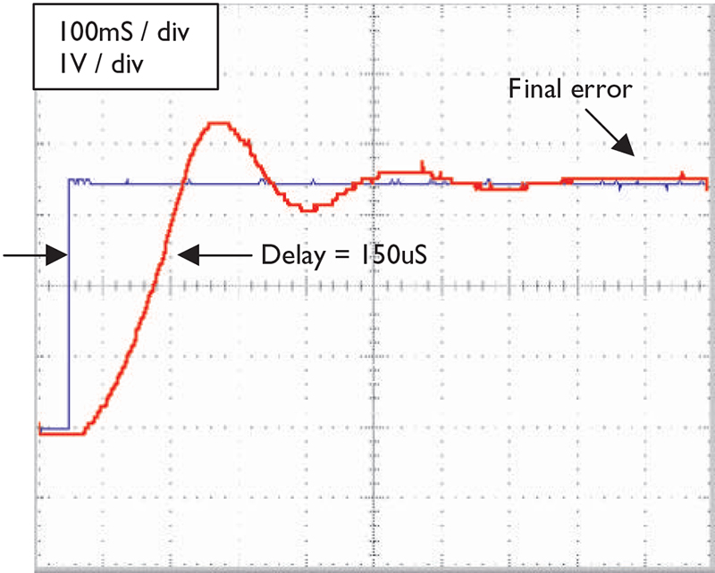
FIGURE 4. Proportional only control has a fast rise time with considerable overshoot and oscillation around the set point: blue = set-point; red = feedback from resistor.
The curve in Figure 4 is a classic example of an “under damped” system. In an under damped system, the system is seen to oscillate about the set point in response to a step input. The system is optimized for rise time. The final steady state error is minimal.
In Figure 5, we see what happens when the proportional gain is lowered.
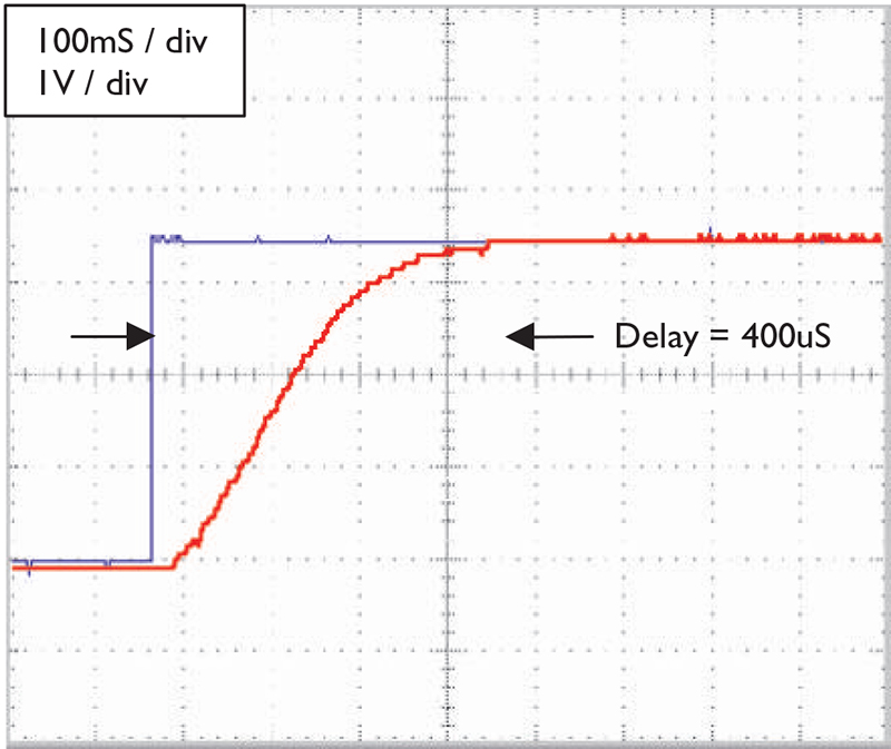
FIGURE 5. The proportional gain is lowered, resulting in a critically damped response and long risetime: blue = set point; red = feedback from resistor.
This figure shows a classic “critically damped” system. The response is as fast as possible without overshoot. If the gain was increased, the system would overshoot and oscillate, as seen in Figure 4. If the gain was lowered, the system would be “over damped” and would take even longer to arrive at the set point.
The critically damped system is optimized for stability. The risetime performance has decreased considerably. To repeat, Figures 4 and 5 show how changes in proportional gain affect the response of the system. For many applications, this type of control is sufficient. However, better response can be obtained with a more complicated system.
Proportional Plus Derivative Control
Recall that the derivative term is a measure of how fast the servo motor is moving. The derivative component is added to the PID result in such a way as to slow the motor down. In Figure 4, we saw how the servo motor bobbled around the set point. Figure 6 shows how the servo motor responds with derivative control added. The resulting system is stable and has a good rise time.
FIGURE 6. Proportional plus derivative control results in fast rise time with no overshoot: blue = set point; red = feedback from resistor.
A close comparison of Figures 4 and 6 reveals how derivative control functions:
- In both diagrams, the initial motor response is identical.
- The overall maximum speed of the motor is slower in Figure 6 (less slope).
- Since the maximum speed is less in Figure 6, the motor does not overshoot.
Just like the proportional control, there is a limit to how much derivative control may be added to the system, but too much derivative control will make the system unstable.
Proportional Plus Derivative Plus Integral Control
To understand integral control, we must first explore the limits of PID control. In Figure 7, we see how the servo motor responds under a load.
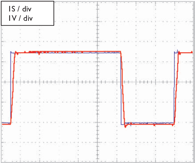
FIGURE 7. Proportional plus derivative control under load. The servo is unable to settle at the set point: blue = set point; red = feedback from resistor.
The servo motor is unable to reach the set point; the blue and red lines do not merge.
From the previous discussion, we know this is a limitation of the proportional terms. We can rule out the derivative term, since it only functions to slow the motor down when it is moving fast. Recall from Part 1 that the proportional system only functions when there is an error.
The simple illustration in Figure 8 will help to explain why the proportional control is not able to eliminate the error.
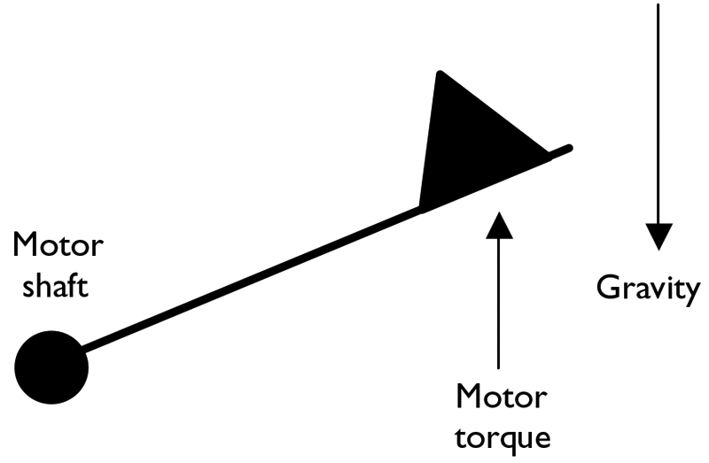
FIGURE 8. A servo motor lifting a weight.
In Figure 8, we see that the motor is holding a weight stationary. Gravity is pulling against this weight. The motor must apply a torque which counteracts the effect of gravity. Without power, the motor would develop no torque and the weight would fall. Recall that the proportional term is proportional to the system error. Therein lies the problem with proportional control.
This one took a while for me to understand, but it makes sense when you think about it. The error cannot be eliminated. If the error was zero, the proportional drive would be zero, and the weight would fall. Therefore, in a set-up such as that in Figure 8, there will always be an error. The blue and red lines can never converge. In Figure 9, we see how the integral component can improve the steady state error of our servo motor system. Recall that the integral accumulates the error over a period of time.
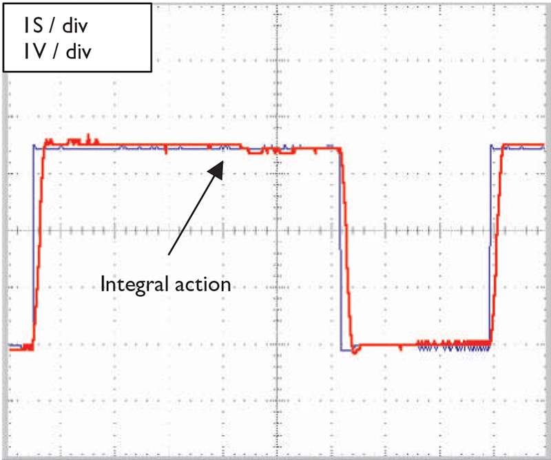
FIGURE 9. Proportional plus integral plus differential control under heavy load. The servo returns to the set point with time: blue = set point; red = feedback from resistor.
In Figure 9, we see that the servo motor has overshot the set point, just like in Figure 7. Since the error is not zero, the integrator will start to accumulate the error. After a period of time, the integrator output is high enough to move the motor, as seen in Figure 8. The steady state error is, therefore, reduced.
To better understand the integral, let’s look at what happens when we increase the integral gain. As you can see from Figure 10, things can get ugly. There are two problems with this system: overshoot and oscillation.
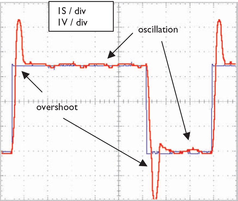
FIGURE 10. Proportional plus integral plus differential control under heavy load. Setting integral gain results in overshoot: blue = set point; red = feedback from resistor.
The overshoot is caused by the rapid accumulation of error. A large error exists for a period of time when the motor is commanded to move. This large error is accumulated by the integrator. This is called “integral wind-up.” If we were to look at the output of the integrator with an oscilloscope, we would see that the capacitor is fully charged, i.e., the integrator has saturated. This is not a good thing! Recall that the capacitor will not discharge until the error has changed signs. This means that the servo motor must overshoot to discharge the capacitor.
The oscillation seen in Figure 10 has an inherent problem with the integrator. The problem is with the very action of the integrator itself. Let me explain with an example:
- Assume an error exists.
- The integrator will accumulate this error over time. Therefore, output of the accumulator slowly rises.
- The motor will move when the integrator output is sufficiently high. The required voltage level is determined by the motor inertia and the mechanical resistance.
- Once in motion, the motor will continue moving.
- In most cases, the motor will overshoot the set point and will start this process over again.
The overshoot is exacerbated by high integral gain. Unfortunately, the effect is also observed with low gains. The system may or may not settle at the set point. However, if the error is zero and the motor is not moving, the system will be in a state of equilibrium and all movement will stop. For the servo motor systems presented in this article, the settling process may take several seconds.
The operation of the integrator may be improved by the additional circuitry shown in Schematic 1. The analog switch we examined earlier helps to stabilize the integral. It does this by disabling the accumulation action if the motor drive is above a particular point.
Figure 11 shows how the system’s performance is improved by adding the analog switch.
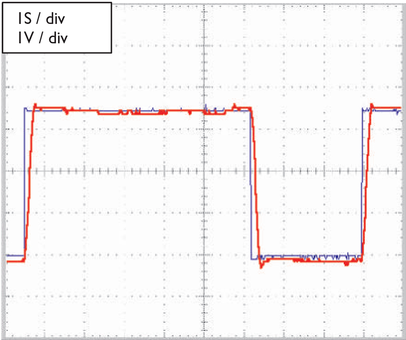
FIGURE 11. Proportional plus integral plus differential control under heavy load. The integral lockout circuit prevents overshoot: blue = set point; red = feedback from resistor.
The integral gain in this figure is the same as in Figure 10. The overshoot has been eliminated; unfortunately, the oscillation remains.
Tuning Summarized
Tuning a PID controller is like riding a bike. You have to keep your eye on system stability, rise time, and steady state error. I have the following rules of thumb to help you:
- Proportional gain determines how fast the system corrects a relatively large error. Increase the proportional gain for faster system response. If the term is too high, the system will overshoot and may oscillate around the set point.
- Derivative gain is adjusted after monitoring the system performance. Increase the derivative gain if the system has a large overshoot in response to step input. If the derivative gain is set too high, the system will again oscillate.
- Integral gain is adjusted to control the performance of the system when it is near the set point. Increasing integral gain will make the system quickly return to the set point. Decrease the integral gain if the system starts to oscillate.
My advice to you is to get out there and try to tune a PID system. We all learn best by doing. The servo motor system presented in this article is very responsive and easy to tune. The lessons learned are applicable to other systems. The worst that can happen is that you will strip a few gears! Also, read, read, read — there are many well-written texts to guide you in this process. As a starting point, I recommend that everyone get a copy of Professor Jacob’s Industrial Control Electronics.
Stay tuned; in Part 3, we will go high tech. We will take the lessons learned in the analog world and apply them to a digital PID controller. NV
REFERENCE
Jacob, Michael. Industrial Control Electronics. New Jersey: Prentice Hall, 1988.
Downloads
PID Controller (includes CAD files)