Let’s review where we have been. In Part 1, we learned what the terms P, I, and D represent. Our discussion was based on analog models, where each component of the PID controller was comprised of a simple op-amp circuit. In Part 2, we learned how the various terms interacted with a mechanical system and we learned how to tune the PID controller for optimal system response.
This time, we are going to take the training wheels off and construct a fully functional digital PID controller. We will be using a ZILOG microcontroller as the brain of our control system, and the same servo motor that was presented in the previous installments will be used. In conclusion, we will compare analog and digital PID controllers.
Microcontrollers
In many ways, this was the hardest section to write. I had to make a difficult decision: What microcontroller platform do I use? My first preference was to use the BASIC Stamp. After all, most of us Nuts & Volts readers are familiar with this processor and it is quite capable. Unfortunately, we need more horsepower to perform the PID algorithm. We also need the performance that can be achieved using a true interrupt service routine.
Obviously, the Stamp isn’t the only microprocessor. There are dozens of manufacturers, so you can take your pick from A to Z: Analog Devices, Atmel, Cygnal, Microchip, Motorola, Rabbit, Renesas, ZILOG ... We could use any of these micros, but luckily for us, one product stands out among the rest. At the very end of the list, we come to ZILOG.
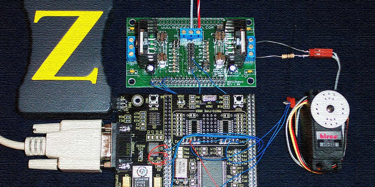
ZILOG is the grandfather of the microprocessor world. They have been around since 1974 (back in the Nixon presidency), and in that time, they have manufactured billions of micros. Their newest Encore! series has just what we are looking for. I rushed out and purchased a Z8642 development kit, and included in this kit is a development circuit board and an in-circuit debugger (shown in Photo 1).
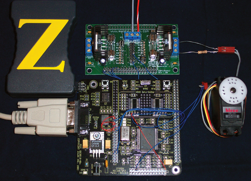
PHOTO 1.
The Z86423 processor mounted on the board has gobs of speed, 64K of Flash memory, 2K of RAM, and powerful built-in peripherals. The kit also includes a full-featured C compiler, all for the price of $39.95! This price is a dream; the last kit I purchased with this many features put me back over $600.00 and frankly, it doesn’t work nearly as well as the Zilog system.
Why Learn C?
If I had to choose a single reason to learn C, it would be that the language is not processor-specific. All of the micros listed in the previous section may be coded in C, as it appears that C is the standard programming language for the micro. With C, you can easily switch to a new micro; you will already know the language. You only need to focus on the hardware differences. With C, you will be able to use code written for one processor on another one. Finally, C is a very powerful language, as it provides high level functions such as floating point math routines and string manipulation. It also allows you to access all of the micro’s hardware registers. If it can be done, C can do it.
We don’t see many articles using C in the pages of Nuts & Volts. Cost is certainly an issue. Up till now, a C compiler for a micro would cost upwards of $400.00. Complexity is another problem, as it exists on two levels. First, the C language itself can be overwhelming and the operations of basic elements are not obvious at first. The language syntax has caused more than one newbie to pull out their hair — all those braces must be in the right places. Second, the microprocessor itself is complex. There are many registers that must be configured before the micro will function.
If you are new to microprocessors and would like to learn how to use C, I have this advice: Don’t try to learn C on a micro! Use your PC. There are hundreds of books available to assist you, and if you are new to programming, you may want to cut your teeth on the Python programming language. Python performs many of its functions in the same way as C does, but it will also force you to use structured programming. Python is available free of charge at www.python.org You may also wish to download the book How to Think Like a Computer Scientist by Allen B. Downey, Jeffrey Elkner and Chris Meyers, from Green Tea Press. Another alternative is to learn using C++. A free compiler is available at www.bloodshed.net The C++ language is similar to C, but skips the stuff on classes and objects.
Once you have learned how to code C on a PC, you can switch back to the micro. The process of learning the micro’s hardware will be much easier if you know how to manipulate the C language. Okay, enough about C. Let’s get back to our main topic and learn how to implement a digital PID using C, naturally.
PID Routine
The PID routine in C has the following form:
void PID_ (){
measure_plant();
calc_error();
calc_proportional();
calc_integral();i
calc_derivative();
calc_PID_sum();
drive_plant();
}
In many respects, this is the same process that was being performed by the analog circuitry. This is a parallel process. The sums of the P, I, and D terms are added together to determine the drive for the servo motor. In this installment, we will use the more generic term “plant” to refer to the process we are controlling instead of servo motor.
The majority of the variables used in this program are external, and by making the variables external (global), they are available across functions. For example, the variable error is first calculated by the function calc_error. It is then used by calc_proportional, calc_integral, and by main.
A base requirement for the PID routine is that the time between iterations must be consistent. If this is not the case, the integral and differential components will appear to have noise and will cause less than ideal operation. This timing requirement is met with an interrupt service routine; we will resume this discussion later in this article.
As written, this PID routine executes in approximately 700 µS (18.432 MHz XTAL). This allows the routine to be executed over 1,500 times a second.
Measure Plant
The first step to implementing a PID controller is to measure the process. We will be controlling the same servo motor as we did in the previous installments. This servo consists of a DC motor with a variable resistor as a feedback element. It is this feedback resistor that must be measured. The Zilog processor has a built-in AD converter to perform this function for us. This Zilog converter will convert an analog signal into a 10-bit number. The input voltage to the converter must be between zero and 3.3 VDC, and if these voltages are exceeded, the micro will be damaged.
The function to measure the plant is shown here. The function get_AD was written to return the 10-bit value of the selected AD channel.
void measure_plant(){
plant = get_AD (ch0);
}
Calculate Error
The second step is to calculate the error. Recall that error is the difference between the desired set point and actual position of the plant measured by the AD converter.
void calc_error(){
error = setpoint - plant;
}
Calculate Proportional
We calculate the proportional component by multiplying the error by a proportional gain term. I have chosen to represent the proportional gain term as integers. If your application requires more adjustment, a float may be used.
Recall that the outputs of the op-amp circuits were limited by the positive and negative voltage supplied to the op-amps. We will perform a similar operation in the micro. The proportional term is limited to an absolute value that is less than or equal to the saturation term.
void calc_proportional(){
proportional = error * proportional_gain;
if (abs(proportional) >= saturation){
if (proportional > 0)
proportional = saturation;
else
proportional = -saturation;
}
}
Integral
Previously, we defined integral as the accumulation of error over time. In the op-amp circuit, we charged/discharged a capacitor. Over time, the capacitor “accumulated” the error. In the digital PID, we will not use a capacitor, but instead, we will use a floating-point register as the accumulator. We will add/subtract the error from this accumulating register every time the PID routine is implemented.
Recall that the op-amp integrator had a resistor that was adjusted to change the speed at which the capacitor was charged/discharged. The charge/discharge speed of the digital accumulator is changed by first multiplying the error by a floating point number. Using this type of operation, we can change the speed of the integrator over a wide range. Also, the speed is dependent on how often the PID routine is executed. Obviously, if the time between iterations is small, the integral term will grow faster.
The integral is limited to an absolute maximum value by comparing it to the saturation term. Also, note that the accumulator is implemented as a static variable. That is, the value stored in the accumulator does not vanish when the function exits.
Finally, a lock-out function is implemented to prevent integral wind-up. This lock-out function is based on the error term. This implementation is different than the op-amp iteration. In the op-amp circuit, we monitored the output of the PID loop. This was possible, since the analog circuit responds more or less instantaneously. This is not the case in the digital implementation. The PID routine is active during a finite amount of time. We could have used the last iteration’s PID output, but this is not ideal, since a large change in the set point would not be seen. This would cause a large error to be integrated, causing integral overshoot: the very effect we are trying to prevent.
Monitoring the error term is a good compromise. For the majority of situations, if the error is large, the PID output will be large. The only problem is that it does not account for the differentiator term. However, if the plant is moving fast, then presumably there is a large error.
void calc_integral(){
static int accumulator;
if (abs(error) <= int_lockout){
accumulator += error * integral_gain;
integral = accumulator;
if (abs(integral) >= saturation){
if (integral > 0){
integral = saturation;
accumulator = saturation;
}
else{
integral = -saturation;
accumulator = -saturation;
}
}
}
}
Derivative
The derivative term is a measure of how fast the plant is moving. If the plant is moving, then the voltage will be different between PID iterations. The faster the plant is moving, the greater the difference between iterations will be.
The derivative term is highly dependent upon the time between iterations of the PID routine. If the time is short, the difference between any two voltage measurements will be small. Likewise, if the time is long, the derivative term will be large. This time between iterations must be constant. If the time changes, the differential term will not be a true measure of the plant speed. Time variation can result in differentiator “noise.”
The actual derivative term is calculated by first finding the difference between the present plant location and the last location. This number is then multiplied by the derivative gain term. Finally, the function verifies that the term is less than the saturation limit.
void calc_derivative(){
derivative = plant - last_plant;
derivative = derivative * derivative_gain;
if (derivative > 0)
derivative = saturation;
else
derivative = -saturation;
last_plant = plant;
}
Calculate PID Sum
After the individual P, I, and D terms have been calculated, they are added together to form the PID_sum term. Actually, the D term is subtracted from the sum of the P and I terms. This is done because the D term is derived from the plant drive. A final comparison is made with the saturation term to ensure that the PID sum term is within the proper limits.
void calc_PID_sum(){
PID_sum = proportional + integral - derivative;
if (abs(PID_sum) >= saturation){
if (PID_sum > 0)
PID_sum = saturation;
else
PID_sum = -saturation;
}
}
Drive Plant
At this point, the PID calculation is complete, and we are left with a value in PID_sum that we will now use to drive the servo motor. This value may be either positive or negative, depending on the required correction. The motor will be driven using one of the ZILOG’s PWMs (Pulse Width Modulators) and an external H-bridge.
The ZILOG micro has several built-in hardware PWMs, which are joys to work with. Since the PWM is implemented in hardware, it is a set-it-and-forget-it device. It operates at relatively high speeds — approximately 18 KHz in this application with 10-bits of resolution. To use the PWM, we configure the appropriate timer, set the period, and set the duty cycle. The hardware takes care of the rest. The PWM will continue to operate automatically in the background until we tell it to stop or change a parameter, which is ideal for our PID routine. We only need to update the PWM once per iteration.
A Magnevation H-bridge is used to drive the motor. This circuit board contains two National Semiconductor LMD18200 power H-bridges, only one of which is used. It is capable of supplying three amps at up to 55 volts. The chip contains current limiting and thermal detection circuitry. Also, the chip is compatible with the 3.3 VDC logic level of the ZILOG processor.
The LMD18200 requires three control signals: brake, direction, and a PWM. The brake line will stop the motor (active high). The direction line will change the rotational direction of the motor, effectively changing the output polarity (sign) of the H-bridge. The PWM line determines the average voltage (magnitude) of the drive signal sent to the motor.
The function drive_plant is responsible for controlling the drive signals to the LMD18200 H-bridge. The basic routine is shown here. The first line of the code disables the motor brake. The if/else pair sets the motor direction (polarity) based on the sign of the PID_sum variable. The final line sets the duty cycle of the PWM to the absolute value of the PID_sum drive variable.
void drive_plant(){
off_PWM3_brake( );
if (PID_sum < 0)
cw_PWM3();
else
ccw_PWM3();
set_PWM3 (abs(PID_sum));
}
Interrupt Service Routine
The timing of the PID routine is important, as the Integral and Derivative functions must occur at precisely timed intervals. Time variations between intervals will show up as noise on the derivative terms and will degrade performance. The actual time between iterations is adjustable (i.e., the Interrupt Service Routine can occur every microsecond or every minute). However, the time interval chosen must be consistent; if you selected a microsecond, then there must be exactly one microsecond between PID iterations.
The best method of implementing these time delays is to use an Interrupt Service Routine. An ISR is like the ringing of a telephone. Normally, we just go about day-to-day activities, but — when that phone rings — it gets our immediate attention. We stop what we are doing and answer it, and the micro does the same thing. Normally, it performs the main line code, but when an interrupt occurs, the micro immediately stops executing the main line code and “vectors” (goes to) the ISR.
The Zilog micro has multiple sources of interrupts. For this application, we are only concerned with timer 0. This timer is set to interrupt the micro every one mS. This results in the code execution shown in Figure 1.
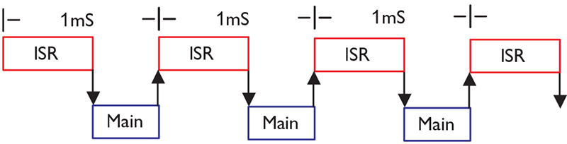
FIGURE 1.
Just like clockwork, timer 0 interrupts the micro. The CPU vectors to the ISR, and the ISR executes the PID routine. When the PID routine is complete, the program returns to the previous tasks.
Setting up an ISR in the Zilog micro involves setting up the timer to overflow every microsecond, enabling the timer interrupt function. Finally, we must tell the micro what code to execute during the ISR. This information is found in the timer.c file, and the demo program included with the Zilog development kit also contains an ISR that you can view. Dissecting this simple demo program is a good way to learn how to operate the micro.
How Do I Tune a Digital PID?
Generally, you can tune the digital PID the same way you tuned the analog PID. The Proportional, Integral, and Derivative gains are present and perform the same functions as they did in the analog implementation. I have added a simple user interface that allows you to adjust the individual parameters via a terminal program. The settings are ANSI, 57600, and 8N1. You will see the following screen:
Welcome to digital PID control with the Zilog Processor.
Select the corresponding number to update a parameter.
1) Proportional gain = 10
2) Integral gain = 0.010000
3) Derivative gain = 50
4) Integral lockout = 700
5) PID Loop time = 1 mS
6) Desired Setpoint = 480
7) For continuous display of the PID terms
8) To toggle the step function
9) To set the step function parameters
time between steps = 5000 mS
high step = 400
low step = 450
To adjust a parameter, type the number you wish to change. Option 7 is particularly useful during the tuning, and if you select this option, you will be presented with the following text:
plant = 500, error = 0, P = 0, I = -46, D = 0, PID_sum = -46
New lines are sent as fast as the micro can process them, and this allows you to see — at a glance — what the PID algorithm is doing. Each of the individual PID components are displayed along with the sum of the PID terms. The plant position and the error are also displayed. This data may be plotted by importing it into your favorite spreadsheet program.
An additional feature that is very useful is the ability to adjust the time between PID loop iterations. I have set the software up so that the loop time may be adjusted between one mS and one minute. This makes the PID adaptable to many different types of systems. For the servo motor, the one mS setting works very well. For slower systems — such as thermal or chemical systems — a longer loop time is desirable.
Be very careful when you adjust the loop time, as small changes can have a profound effect on the integral and derivative gains of the system. I lost most of the servo motor gears by making this mistake! Remember those limit switches?
Analog Versus Digital
The digital PID controller produces results that are on par with the analog system, as seen in Figure 2.
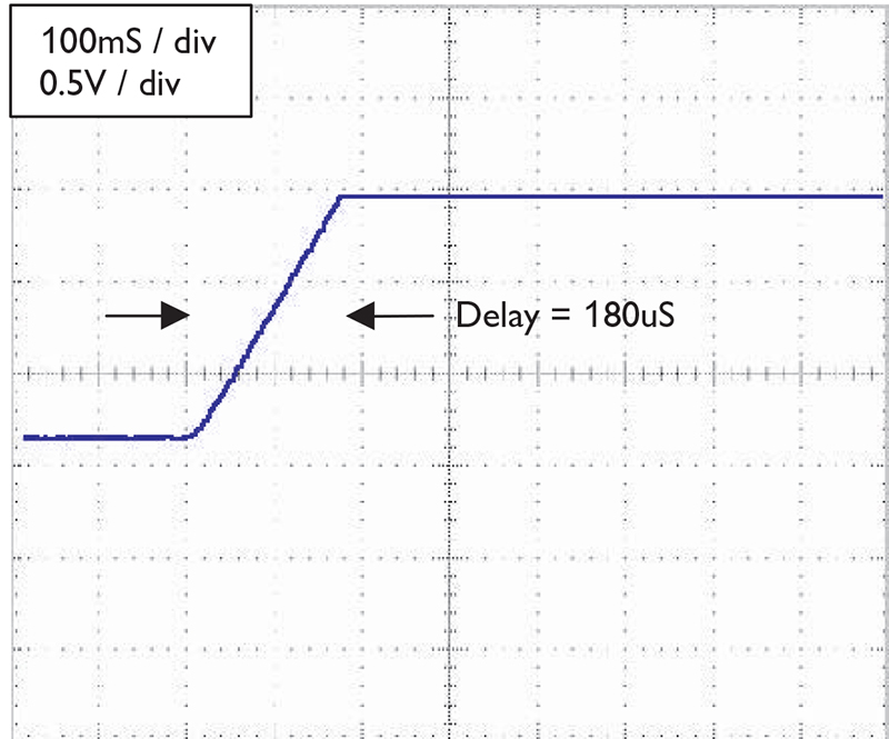
FIGURE 2.
I have observed that the derivative component of the digital controller is more responsive. The derivative gain may be set higher, thereby minimizing overshoot. The rise time is also improved, which may be attributed to the higher voltage applied to the motor.
It is tempting to state that the digital PID is superior to the analog system. After all, isn’t digital the wave of the future? It turns out that determining which is the best PID controller depends on the application in question.
- If you have a fast system, then use the analog PID. An example of a fast system is a power supply or a high-speed motor.
- Conversely, if you have a slow system, then use the digital controller. Thermostatic control is an example of a slow system. It is difficult to make an analog integrator or differentiator that will function at these long time constants.
- For general-purpose control in a variety of situations, digital control is preferrable. The ability to make adjustments in software is much easier than having to change hardware.
- The digital system is preferred for high power systems. The PWM output scheme is more efficient and scalable.
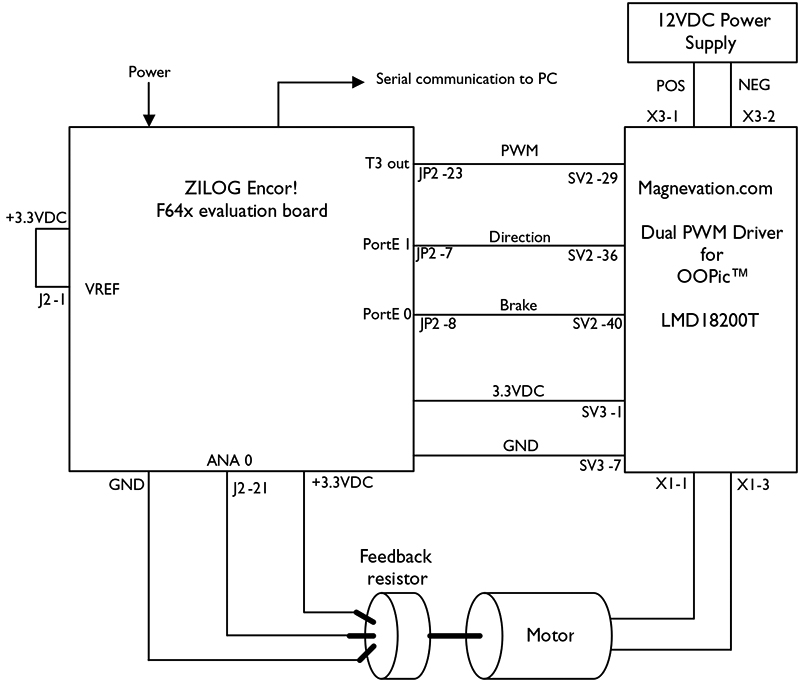
FIGURE 3.
Next Step
In this series of articles, you have used a simple servo motor and the “plant.” The servo motor provided a good starting point for the PID, since it is a relatively slow system that is easy to see in operation. The next step is to adapt the lessons learned on the servo motor to new applications. A few examples come to mind:
- Improve the servo motor. At best, a resistor is a poor device to use to measure position in a mechanical system. It has poor resolution, is susceptible to noise, and has limited life. A better solution is to use a non-contact measurement system. A quadrature encoder mounted on the motor would have more resolution, less noise susceptibility, and longer life.
- Change the measured parameter. In this article, we have focused on controlling the angular position of a servo motor, and the methods and ideas may be applied to measure distance traveled. A PID controller is a natural addition to a robot.
With the PID, you could measure the distance the robot has traveled, and you could control acceleration. Your robot would have the ability to operate on an incline, since the integral control would keep your bot at the desired position.
- Digital control of a PWM power supply: This application was mentioned in Part 1. A PID controller would allow you to control the voltage and current of a power supply. If you really want a challenge, try to construct a maximum power point tracker.
- Thermal control: The digital PID is capable of controlling a system with long time constants. This makes it an ideal platform for controlling thermal systems. A digital thermometer — such as the Dallas DS1624 — could be used as the sensing element. This combination would produce an accurate thermostat.
With this new information, you are well on your way to producing high-performance control systems, and I hope you find control systems engineering as exciting as I do. The training wheels are off. Go find out where the PID can take you! NV
Downloads
PID Controller 2005-04 (program codes)