Turn Your 16-Bit Micro Experimenter Into A Powerful Digital Signal Processor!
By Thomas Kibalo
Since the Experimenter is socketed, the change in hardware is straightforward. For software, the dsPIC is supported by the free Microchip’s full function ’C’ based DSP software library.
The dsPIC is pin to pin compatible with the PIC24F part that comes with the 16 Bit Micro Experimenter Kit; however, but there are significant enhancements. The dsPIC has built-in Digital Signal processing hardware, supports 128K of Flash and can operate up to 40 MIPS. In addition, the dsPIC supports all the PIC24F peripherals, and supports a 12 bit ADC, a DCI (Digital Communication Interface) interface, Dual DAC (Digital to Analog Convertors) and a built-in DMA (Direct memory Access).
A DSP notional system block diagram is shown in figure 1. The actual prototype is shown in figure 2.
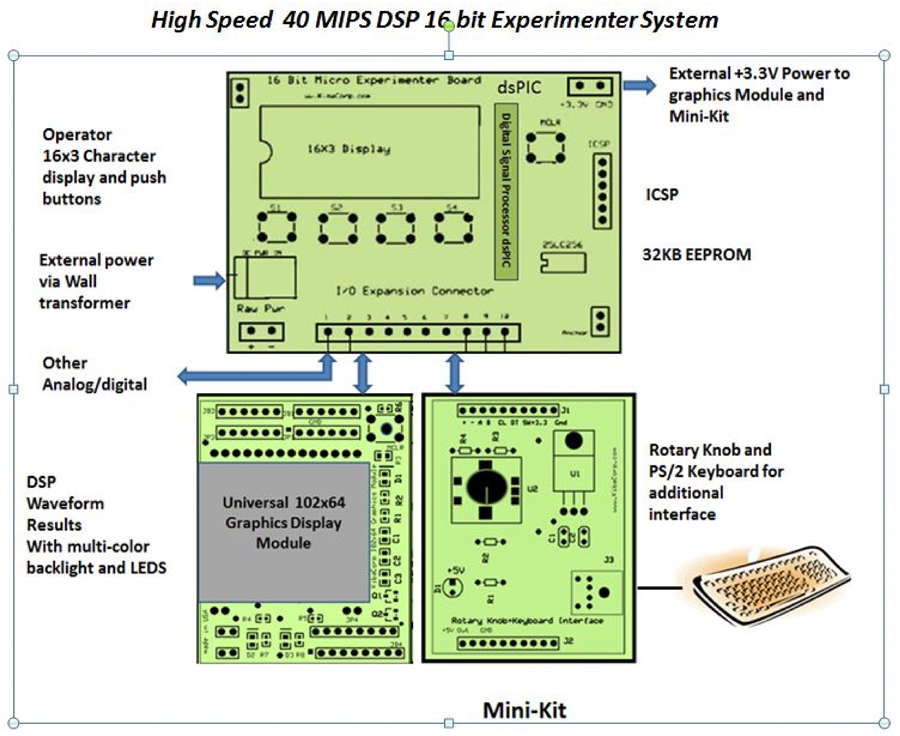
Figure 1 DSP Experimenter Block Diagram
Why Digital Signal Processing?
DSP is one of the powerful technologies shaping science and technology at this time. It directly impacts a broad range of applications; brushless motor control, high fidelity music, medical imaging, HDTV, speech synthesis and sensor data acquisition. DSP is distinguished from other areas in microcontroller applications, in that, it uniquely process signals as data.
We are introducing DSP for the Experimenter in a series of Digital Signal processing (DSP) experiments. These are highlighted in the new CD ROM “16 bit Micro Experimenter Handbook” for sale on Nuts and Volts website. The first of these experiments is to perform a real time Fast Fourier Transform (FFT).
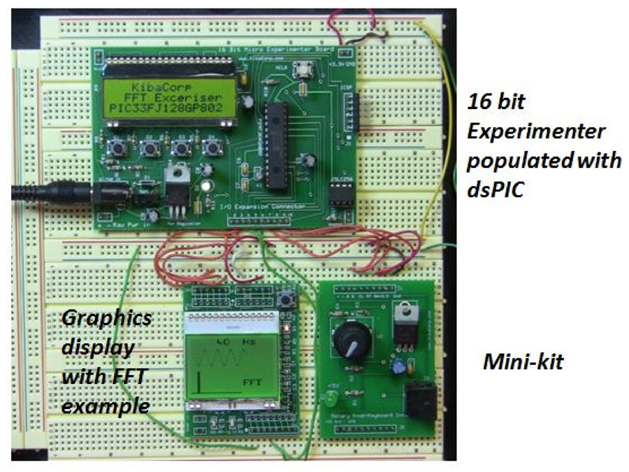
Figure 2 Actual DSP Experimenter Prototype w/o Keyboard
Using The Fast Fourier Transform (FFT)
The FFT is one of most important tools in digital signal processing. It allows us to process a signal and completely determine its frequency composition or spectrum.
Our example takes 128 points of an internally generated sine wave (sampled at 640Hz) and executes a 64 point FFT using Microchip DSP library. These 64 points are then converted and displayed as 32 discrete frequency bins to represent the entire signal’s spectrum. The spectrum bin size in our example is 10 Hz, so the signal’s complete discrete frequency content is displayed from DC to 320Hz in 10Hz increments. It's like having your own spectrum analyzer!
The generated sine wave is default to 60Hz. This is shown as 128 points on the graphics display. For the display we are using the Universal 102x64 Graphics Module. To make things interesting we allow for signal frequency to change between FFTs. For this we use a rotary encoder. The rotary encoder captures position/rotation which can be converted into increment frequency for changes in either direction from an initial 60 Hz setting. The Mini-kit provides the rotary encoder interface. Both the Mini-Kit and Graphics Module are also available from the Nuts & Volts web store.
The application continually performs an FFT displaying both the signal and its associated spectrum. Graphic displays are shown for 40HZ, 44HZ, 46HZ and 50HZ test cases. Note that at both 40 and 50HZ a single bar appears as spectrum, this is because the bin size is 10 Hz, and the incoming signal fits nicely into 10HZ bins. In other cases like 44 and 46HZ the spectrum does not fit “neatly” into a single bin and “spills over” into adjacent bins. This is exactly how an FFT performs.
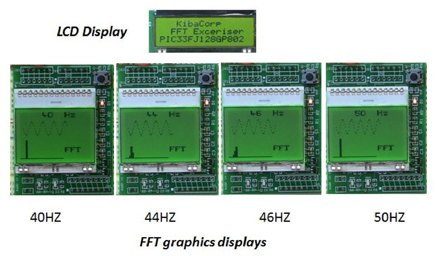
Figure 3 FFT Display Examples
The FFT is a notoriously complicated algorithm but Microchip’s DSP library makes it straightforward. See code segment below (figure 4) the main software loop is shown. The main loop builds the sine wave, populates it to an input buffer which the FFT crunches on. The FFT results are then converted to magnitudes which are then displayed.
while (1) {
makewaves(); // Synthesize SINE Wave
clearScreen();
plotsignal(&temp, 64,5,-10); // plot SINE wave
AT (4,0)
sprintf (s, “%d”, freqa); // output Frequency value
putsV (”Hz”);
line (0,63,63,63) ;
AT (8,6)
putsV(”FFT”);
dumpVmap();
for (i=0; i<REAL_N; i++) //populate input buffer with SINE values
ipFftBuff[i] = ipFftBuff[i] <<16;
// Do FFT
FFTReal32bIP(REAL_LOGN, REAL_N, ipFftBuff, psvTwdlFctr32b, _builtin_psvpage(&psvTwdlFctr32b))
// create FFT Magnitude
MagnitudeCplx32bIP( ( REAL_N/2)+1, ipFftBuff);
for (i=0; i< NUM_SAMPLES; i++)
Ltemp [i] =0;
for (i=0; i <NUM_SAMPLES/2; i++)
Ltemp[i] = ipFftBuff[i] >>16; //create INT for frequency plot
plotFFT (&Ltemp, 32,0,63); // plot FFT on screen
dumpVmap();
delay_40msec();
}
Figure 4 Main Code
Code Download FFT_Demo_ver3.zip
You will need to also install a free version of Microchip's DSP DSC to compile the demo software. A hookup diagram for our DSP system is provided.
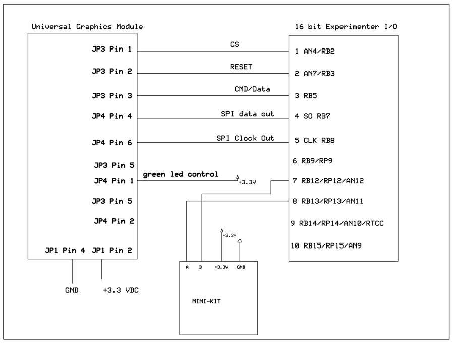
Figure 5 Hook-up
In subsequent feature articles we hope to present even more DSP experiments Digital Filters, Signal Synthesis, Voice Synthesis until then Happy DSP computing! NV
Comments