Last time, we showed you how to connect an Arduino Uno to MakerPlot in order to plot a single channel of analog data using a 10K potentiometer to generate the variable voltage readings. We also showed you how MakerPlot can scale a microcontroller's raw 0 to 1023 A2D (analog-to-digital) output values into corresponding 0 to +5 volt levels — without resorting to coding the conversion math in the sketch. This time, we're going to show you how to add digital signals for plotting, as well as demonstrate how to play back both the analog and digital data in the plot area. Then, we'll show you how to data log what's being plotted to an Excel file for later analysis. If you haven't already done so, download the free 30 day trial copy of MakerPlot from www.makerplot.com to follow along. Let's get going.
Arduino Hardware Setup
Figure 1 illustrates the Arduino Uno with an attached 10K potentiometer.
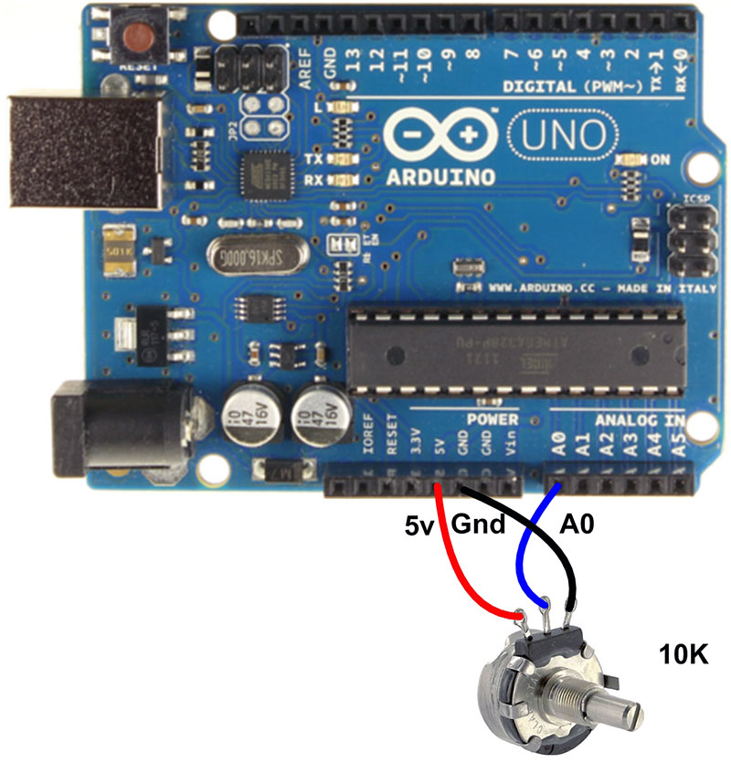
Figure 1. Arduino Uno setup.
This hardware setup can plot a single channel of analog data. However, MakerPlot is capable of plotting up to 10 analog channels, so you’re able to plot all kinds of analog inputs like audio signals, light sensors, thermisters, heart rate monitors, etc. — all at once. For this example, we’ll keep it simple at one analog input for the pot.
Generating Digital Signals
MakerPlot is capable of plotting digital signals, too. Figure 2 is a sketch for generating digital data along with the single channel of analog data from the potentiometer. While MakerPlot is capable of plotting up to 32 digital channels (bits), we’ll plot just eight to show the concept.
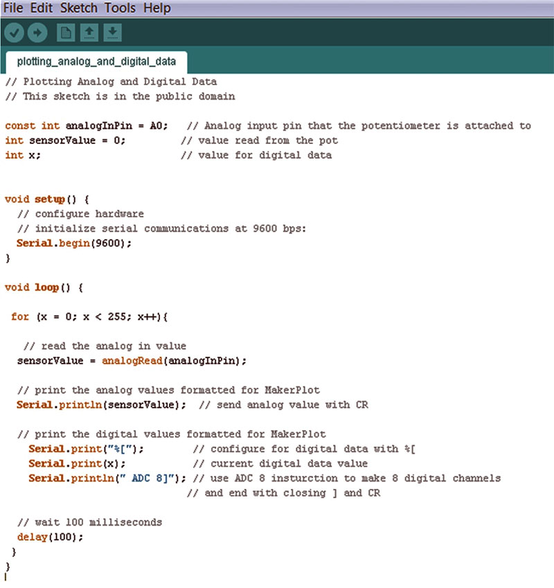
Figure 2. Arduino sketch.
This is how it’s done. Referring again to Figure 2, you can see that we added the variable x that’s used in a For Loop with values between 0 and 255. We did this in order to produce the eight channels of digital data. Here’s the part of the code that outputs the ASCII digital data. It’s separated into three lines for a purpose. Notice how the entire string is bounded by double quotes (“ “); this is important so that the resulting data within the quotes are translated into ASCII:
Serial.print("%["); // configure for digital data with %[
Serial.print(x); // current digital data value
Serial.println(" ADC 8]"); // use ADC 8 instruction to make 8 digital channels and end with closing] and CR
In the first line, MakerPlot uses the percent (%) sign to distinguish what follows as digital data. Next, comes a square open parenthesis ([) that MakerPlot uses to bound the variable. The next line is the value x that produces the digital output. That, in turn, is followed by the MakerPlot instruction ADC 8 that tells MakerPlot to generate eight channels of digital data from the x value. Then, we round out the data set with a square closed parenthesis (]). The Serial.println instruction also terminates the analog and digital strings with a Carriage Return character which MakerPlot requires to know when the data for this field is complete.
Now that the sketch is complete, we’ll copy and paste it into the Arduino IDE (Integrated Development Environment), verify it, then load it into the Uno. Then, we’re ready to do three other things:
- Plot the analog and digital data.
- Replay it in the plot area.
- Data log it.
Plotting Analog and Digital Data
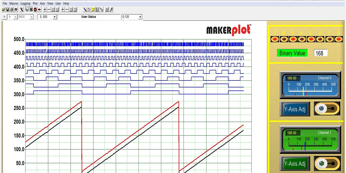
For this sketch, we’re going to choose the MakerPlot Digital Interface (Figure 3) since it plots both analog and digital signals, with the emphasis on digital plotting.
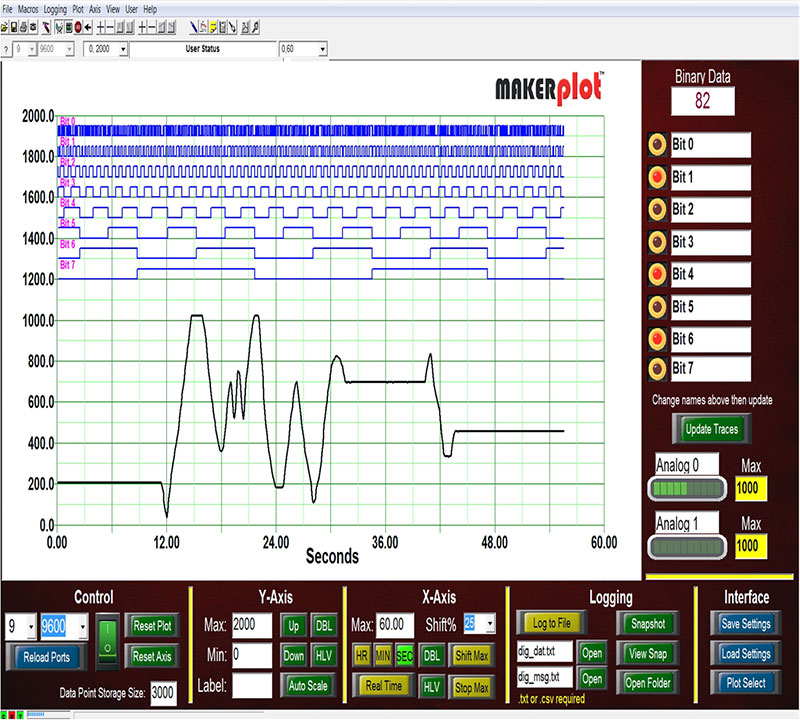
Figure 3. Digital interface plotting analog and digital data.
With the Uno physically connected to the PC via the USB cable, we’ve clicked on the rocker switch at the bottom-left (under Control) to begin plotting the data. As you can see, the digital data are at the top (LSB first) and the analog (potentiometer) data are on the bottom. The pot shaft has been adjusted back and forth to generate a data plot.
The vertical Y scale is between 0 and 2000 to accommodate the raw A2D data going from 0 to 1023. The Y scale can be changed to any value you choose using the menu controls on the bottom. You can also witness the analog data as Analog 0 in the bar graph on the right side of the plot (Figure 4).
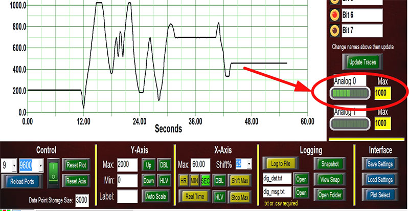
Figure 4. Analog 0 bar graph.
The horizontal bar graph range is currently set to 1000, meaning each one of the 10 LED icons that make up the bar graph is worth 100 analog units. Like the Y scale, you can change this value to anything you wish — including changing the title from “Analog 0” to, say, “Pot Value.” Just key in the new range (1023) and title (Pot Value), and that’s it! Figure 5 shows the results of this customization effort.
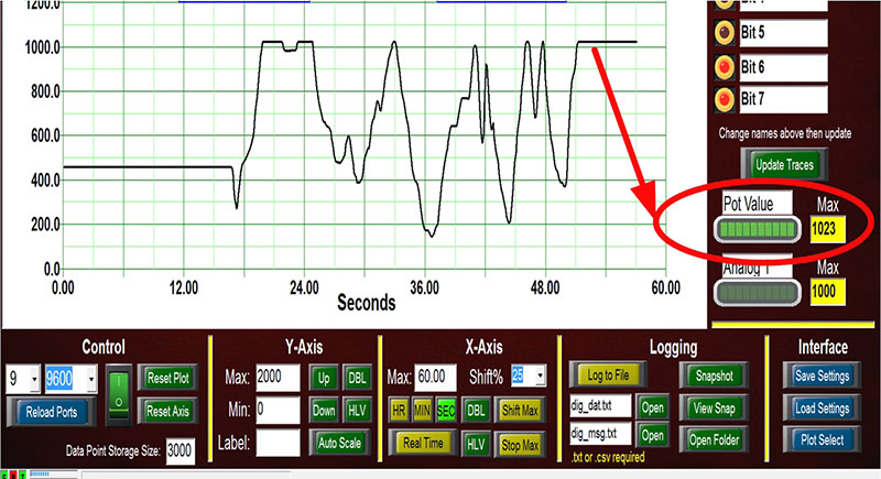
Figure 5. Adjust bar graph and range value.
The vertical Y scale has no real meaning for the digital data since each channel or bit of digital data simply plots along successive horizontal grid lines — in sequence — from LSB (top) to MSB (bottom). Also notice that each digital trace is labeled as bit 0 through bit 7 — both on the left side of the plot area and also right next to the LED that corresponds to the digital data channel on the right (Figure 6).
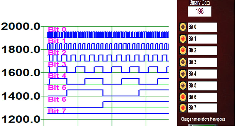
Figure 6. Digital channel text annotation.
Like most everything in MakerPlot, these designations can be changed to whatever you want; you can name each digital channel to represent its meaning within your data monitoring setup. For example, the first and last channels to represent the LSB and MSB of the bits have been relabeled (Figure 7).
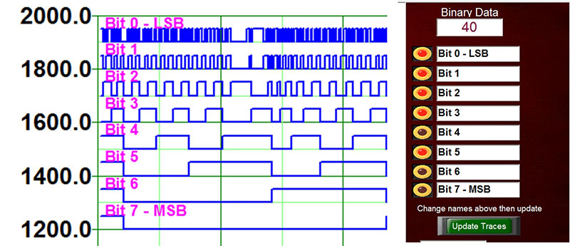
Figure 7. Revised annotation.
Just key the new names into the text boxes next to the LEDs, then click the Update Traces button below. It’s that simple!
Playing Back Data
Now that we have analog and digital data plotting, let’s show you how to replay the last 3,000 data points so you can better analyze it. The playback “capture” is based on the Data Point Storage Size indicated in the Control menu area (Figure 8). Of course, you can change this value up or down to suit your recording needs; the larger the number, the greater the number of data points captured.

Figure 8. Data Point Storage Size.
However, the larger the number, the longer it takes for MakerPlot to refresh the plot area. Practical Data Point Storage Size values range from 500 to 50,000 with 3,000 being the default. So, for this example, we’ll leave it at the 3,000 default setting.
The captured data — which is based on the Data Point Storage Size — is cleared when the plot resets as it gets to the right-end of the plot area. So, to execute a recording, first let the plot run from left to right and “nearly” to the full length of the plot area — but not all the way. Just before it gets to the end, click the green rocker switch (Control menu) to disable the connection between the Uno and MakerPlot.
For this example, the rocker switch was clicked to red (OFF) about 50 seconds into the plot, and just before the plot reached the right-hand side where it gets reset. Next, the Player icon in the Toolbar was clicked (the one that looks like a “hand and wand”), which brought up the Player control (Figure 9).
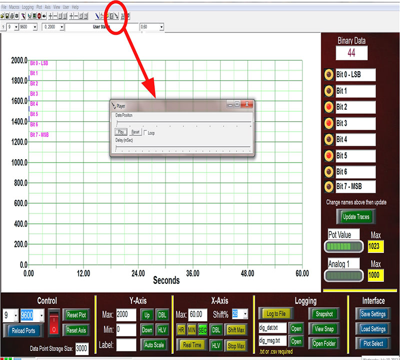
Figure 9. Bring Up Player tab.
So, now with a clear plot area and the Player control displayed, here’s how to replay the last set of captured analog and digital data.
Click on the Play button inside the Player control. This will start the data playback (Figure 10). The Play button changes to Pause, meaning that you can click it again to halt the playback in order to examine a particular area or point in the plot. Clicking it again resumes the playback.
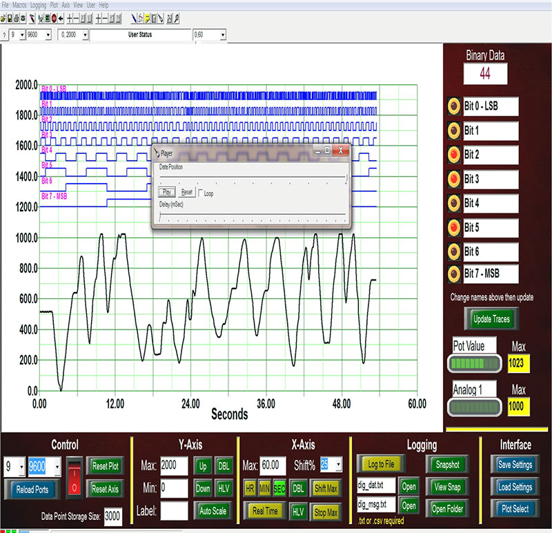
Figure 10. Data replay.
You can see the progress of the playback by looking at the Data Position slider arrow — AND — you can place your mouse cursor on the Slider arrow to move it back and forth which allows the plot to replay up to the point where the slide arrow comes to rest. Plus, you can click the Loop check box for continuous play.
To slow things down, you can place your mouse cursor on the Delay arrow and move it to the right which adds the indicated millisecond delay between plotted data points. Try it. With enough delay, it will give you a “burst by burst” plot of the recorded data so you can stop it wherever you like with much better control.
So, that’s how to use the Player function to replay data for immediate review. Now to data logging in Excel CSV format.
Data Logging
With data logging in MakerPlot, you’re not limited to the last 3,000 or so data points; you can log any amount of analog and digital data that you choose for as long as you choose — minutes, hours, days, etc. — to either a text file or a CSV file. Remember, you’re basically saving a text file to a computer hard disk and not just a few memory chips on your micro’s board. So, there are no practical memory-limiting issues to worry about when data logging with MakerPlot. Here’s how it’s done.
First, take a look at the Logging menu at the bottom in Figure 11.
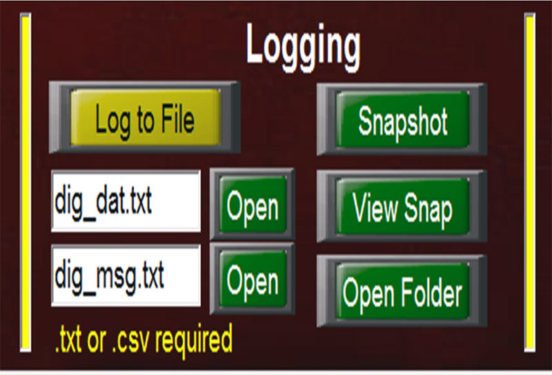
Figure 11. Logging menu.
On the left side, you’ll see the Log to File button and below it, two text boxes with file names. The first text box is for logging data and the bottom text box is for logging messages. Messages, by the way, are an important alerting feature since you can program MakerPlot to output messages based on certain data levels or combinations, and then you can log these messages with date and time stamps for later analysis. We won’t be getting into logging messages in this example; however, just be aware that you can.
The default data text file is dig_dat.txt which means that logged data will be sent to this file name which — by the way — is a standard text file with a .txt extension. We’ll change the file name and extension to reflect logging our analog and digital data to the CSV file. Once again, this is easily done by simply clicking on the text box just below the Log to File button and keying in a new file name. The one chosen is called ana_dig.csv (Figure 12). With that done, let’s log some data.
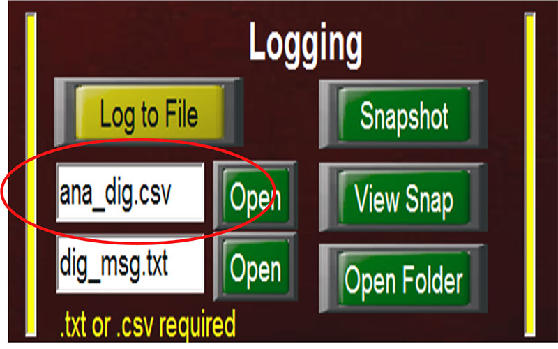
Figure 12. Logging menu with new file name.
Click the red rocker switch in the Control menu to start the data flowing into MakerPlot. Now, click on the Log to File button which will change from yellow to green. As long as it stays green, every data packet from the Uno will be logged and time stamped. Let a few seconds go by and then click the Log to File button again; this ends the data logging session. Now, let’s look at what got logged.
Click on the Open button next to the ana_dig.csv text box. This brings up the NotePad file of the logged data (Figure 13).
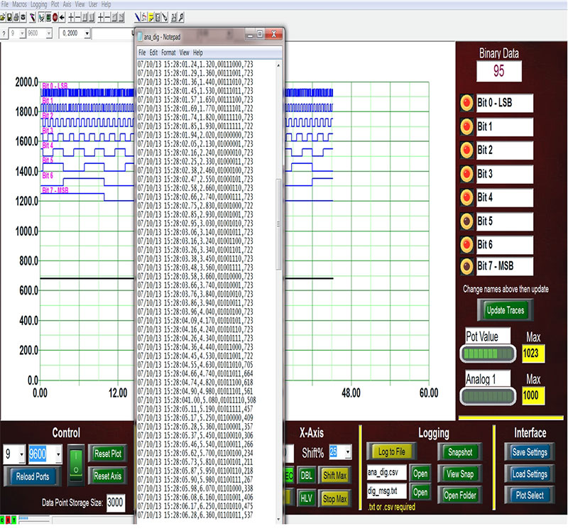
Figure 13. Logged data in NotePad.
Here, we can examine the logged data in some detail. Looking at the first record (Figure 14), we see that the numbers on the far left represent the date and time (with time down to hundredths of a second). This is followed by the time into plot (in thousandths of seconds) followed, in turn, by the state of the eight digital data bits (MSB to LSB), then is followed by the analog value of the potentiometer. If there were more analog channels for logging, they would follow this one. As you can further see, these individual fields are separated by commas which will allow for direct transfer to Excel.
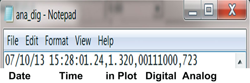
Figure 14. Typical data log record.
Where, you might ask, is this file on the hard disk? When you install MakerPlot, the default location is My Documents → MakerPlot → Data which is where you’ll find it. Just make sure to turn on your file extensions to see the .csv extension. You can now load the ana_dig.csv file into Excel for any type of analysis.
We’re not done with what MakerPlot can do with this file just yet, so let’s show you a few more interesting things.
Displaying Logged Data
To display the logged data, let’s first turn off the data flowing from the Uno by clicking the green rocker switch in the Control menu. Next, click on Logging on the top line, followed by Plot From Data Log. Then, click Open (Figure 15).
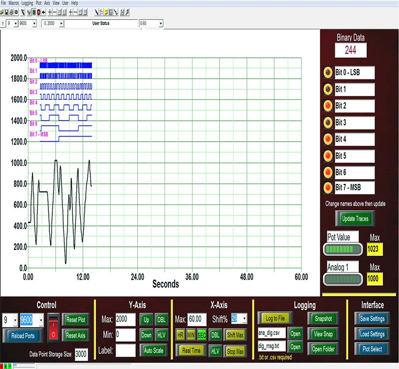
Figure 15. Plot of logged data.
What you’ll see is the logged data plotted just as it was recorded.
Playing Back Logged Data
Going back to the Player function, you can replay the logged data just as before, but this time we’re replaying logged (not real time) data (Figure 16).
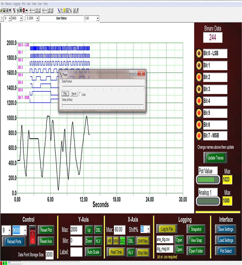
Figure 16. Playback of logged data.
This gives you an opportunity to examine the logged data in graphic detail. You can also expand or contract the time axis using the DBL and HLV buttons to your liking. You can shift the plot left and right with the arrow keys on the Tool Bar, as well.
There are videos on the MakerPlot website that show you all about the Player function and data logging features. Just go to the MakerPlot website (www.makerplot.com) After you arrive, just click on More → then Videos → then Basic Plotting → then the Player Tab and Logging Menu to view all that can be done (Figure 17).
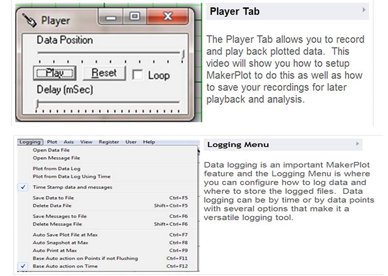
Figure 17. MakerPlot video tutorials.
These short videos will give you a much better idea of these features than we can do here in just a few words and figures, so be sure to check them out.
Conclusion
Let’s review what we’ve covered and what’s coming up in the next article.
We learned how to plot both analog and digital data from the Uno, followed by playing it back using the Player function. We also learned how to log the data and play it back on the plot area for greater analysis. Finally, we showed you how to configure the data logged file name with a .csv extension so it can be ported directly into Excel.
In the next article, we’ll continue to expand on our Uno setup to show you how you can add two pushbuttons and an LED to your Uno board in order to begin doing some interesting bi-directional control experiments. This will take more than just one article to address as it covers a lot of ground; however, it will be worth it since you’ll begin to understand how MakerPlot can act like a front panel for your microcontroller projects with switches and other controls that can manipulate your micro’s actions. NV