What You Don't Know about Your Power Source may be the Problem!
Typical Power Sources
With few exceptions, every electronics project needs a power source. It’s what makes the electrons go round and round. However, not all power sources are created equal.
Too much voltage noise can screw up analog measurements. Not being able to deliver enough current when you need it means your project fails. A transient voltage drop may cause something else in your build to fail — the hardest sort of problem to debug. Delivering too much current when there is a malfunction usually means smoke is in your future.
If you know the requirements of your application and — more importantly — the characteristics of your power source, you can avoid these problems and have confidence. If there is a problem, at least it’s not with your power source.
In this article, we look at four common sources of powering a project:
- Wall Warts
- Batteries
- USB Power
- Arduino Digital Pins
Even among the same type of source, there can be very big differences in their properties and performance. Let’s look at the most important features we should care about for any power source, how to measure them, and what to expect.
The poster child we’ll use to explore the properties of a power source is a 12V wall wart, shown in Figure 1.
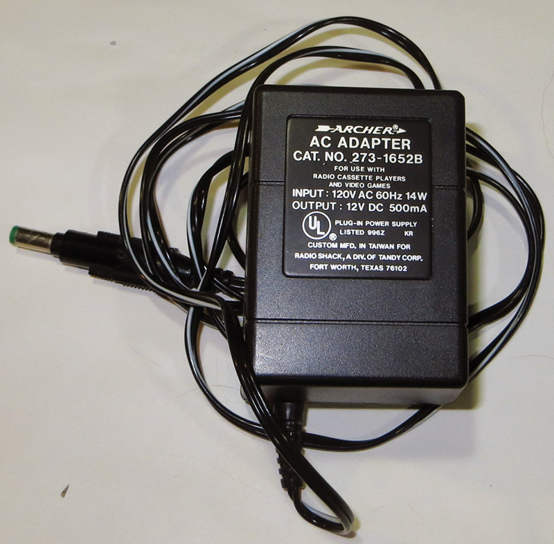
FIGURE 1. A 12V wall wart used in these early investigations.
We’ll use it to illustrate the tests we’ll run, and analyze the features to look for. Then, we’ll apply these tests to the other types of sources and look at what to expect. You will never look at a power source the same again.
Not All Wall Warts are the Same
Almost every low cost consumer product today uses an external wall wart as its primary power source. The output is usually a DC voltage from 5V to 30V. If you get rid of the original product, don’t get rid of the wall wart. Re-use it for your next project.
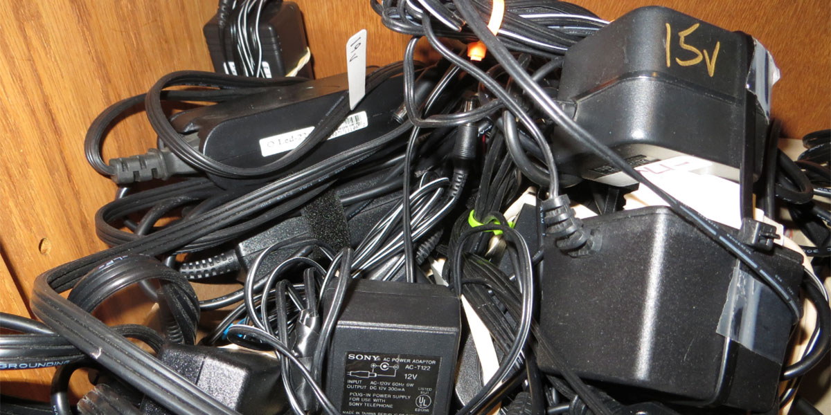
I have a box of extra wall warts I’ve been collecting, and use them over and over again. Figure 2 shows some of that collection.
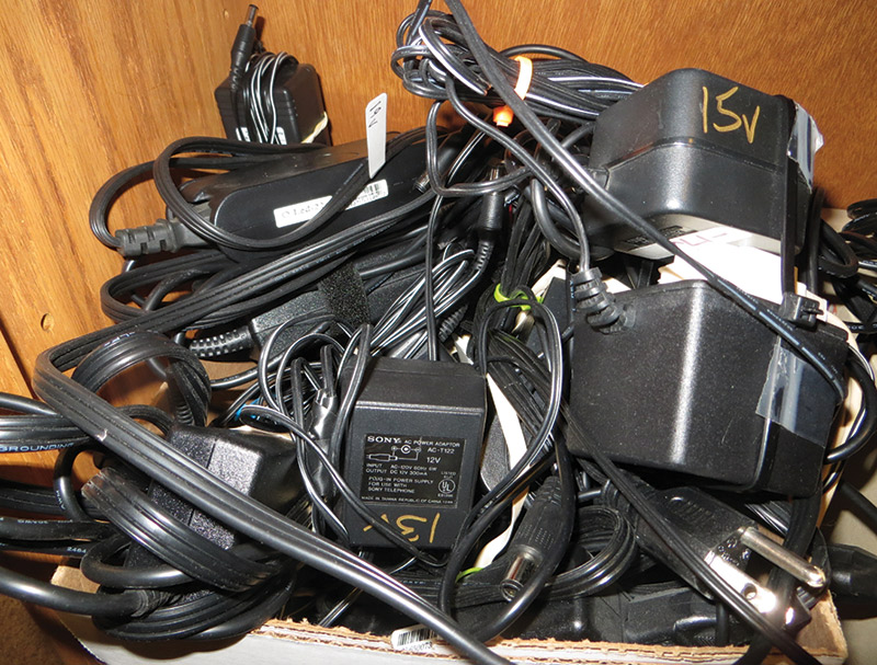
FIGURE 2. A selection of some of the wall warts I’ve collected and reused for my projects.
Look on the outside of any wall wart and you will see a rating for the DC output voltage and the current rating. You can see some of these values in the figure. Don’t take these numbers too seriously. They are more of a guideline. Before you use the wall wart — or any power source — you’ll want to characterize it using the tests described here.
I grabbed one of these wall warts that had 12V output/500 mA stamped on its side. We’ll also look at what this really means and why this doesn’t tell the whole story.
Voltage Properties
To test the properties of a power source, we need to be able to measure the voltage at its output not only when it is unloaded, but also when a resistive load is attached which would draw comparable current as with the intended application.
What we want to look for is the DC voltage levels and the AC noise — usually in the form of 60 Hz or 120 Hz ripple. The best way of doing this is using two channels of a scope. If you only have one channel available, use it to measure the AC ripple and use a digital multimeter (DMM) to measure the DC voltage.
The AC coupled mode of the input to a scope is the perfect setting to use to look at 60 Hz or 120 Hz noise on the power supply voltage.
My personal favorite scope for general lab applications is the Digilent Analog Discovery scope. It has two channels — each with 14-bit vertical resolution — 100 Msamples per second, and an excellent user interface. I can add a math function which can calculate the average voltage — even the peak-to-peak voltage. On top of that, you can do an FFT (Fast Fourier Transform) of the measured voltage signal to look at the spectrum of the entire waveform.
The system I used to perform the voltage measurements in this article is shown in Figure 3.
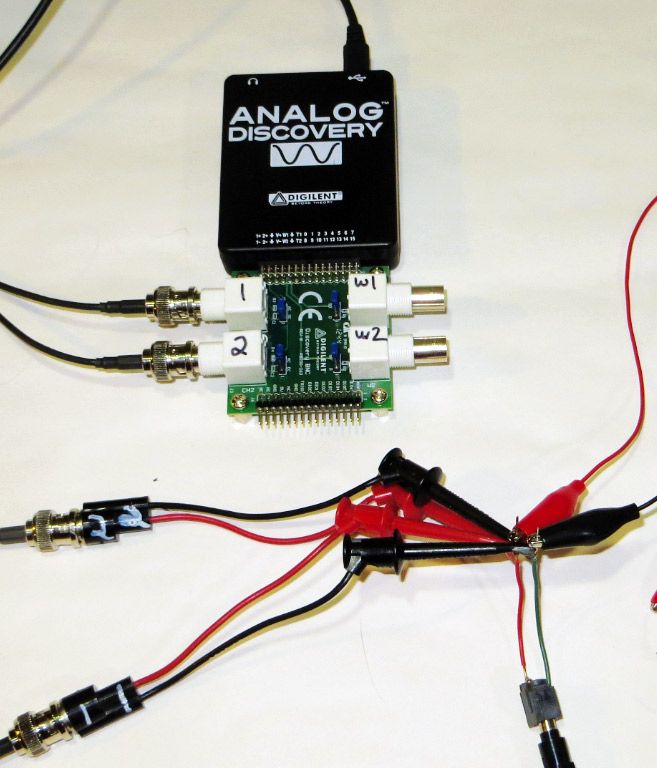
FIGURE 3. Analog Discovery scope with two channels connected to measure the voltage on the power rail.
The scope is set up to measure the unloaded voltage from a wall wart, using a simple power plug to connect to the wall wart. Channel 1 was set for DC, 1 megohm input, and channel 2 was set for AC coupled input.
The measured DC and AC ripple from this unloaded wall wart is shown in Figure 4.
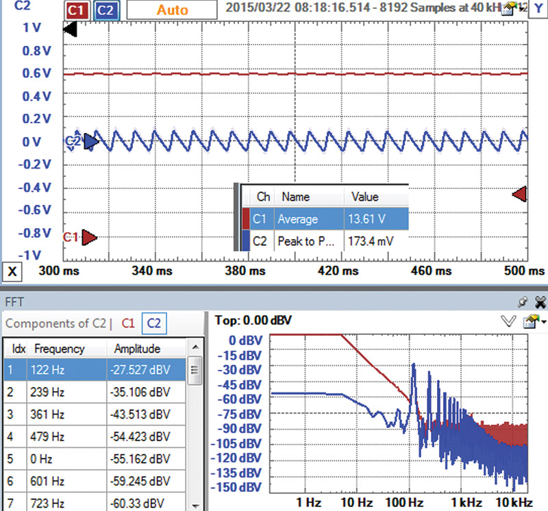
FIGURE 4. Screenshot from the Digilent Analog Discovery scope customized to show the DC voltage, the AC voltage, the average voltage, peak-to-peak voltage, and the FFT of the AC ripple signal.
The scope’s user interface allows me to customize the information displayed to quickly get me the answer I’m looking for.
While the rated voltage is 12V, we see the measured average voltage is actually 13.61V. There is also clearly some AC ripple. In fact, the scope measures 0.173V of peak-to-peak ripple. This is a noise of about 1.3%. The DC and peak-to-peak values are read right off the math functions of the scope interface.
How to Read an FFT Spectrum
In addition to just the voltage over time measurement, I set up the scope for an FFT analysis of the AC ripple signal. We see the waveform in the time domain is triangular, with a repeat frequency of 120 Hz. This is from a full wave rectified 60 Hz source, so it repeats every 120 Hz rather than every 60 Hz.
When we take a triangle wave and look at its spectrum, we see all the harmonics — multiples of the first fundamental frequency — with amplitudes that drop off with frequency. The spectrum shows all the peaks plotted on a log-log scale. The first harmonic is 122 Hz, the next is 239 Hz, and then 361 Hz. They are not exactly 120 Hz and its multiples because of the time window I used. With a time base of 200 msec full scale, the resolution of the spectrum is 1/0.2 sec = 5 Hz. To within 5 Hz, they are 120 Hz, 240 Hz, and 360 Hz.
The highest frequency measured is related to the data sample rate of the scope. The Nyquist Theorem says that the highest sine wave frequency component that can be measured is half the data rate if the signal has a random noise component.
In this example, the sample rate was 40 kHz (displayed in the upper bar along the top of the screenshot), suggesting the highest frequency sine wave component we can measure is 20 kHz. This is a perfect frequency range to evaluate the ripple noise on the power supply.
The vertical scale is the amplitude of each sine wave component. I set the scale to be in dB. To convert the dB value into a voltage amplitude, we take the dB value, divide by 20, and put this to the power of 10.
The peak value of -27.5 dB for the 122 Hz component is really a voltage amplitude of 10^(-27.5/20) = 45 mV. However, we measured a peak-to-peak value of 173 mV in the time domain. Taking half of this as the amplitude would be 87 mV — almost twice the 45 mV we get from the spectrum.
This difference is because in the time domain, we measured the total peak-to-peak value of the triangle wave; while in the frequency domain, we are looking at the sine wave frequency component amplitudes.
The first harmonic amplitude of this triangle wave is 45 mV, but there are a bunch of other amplitudes in the spectrum — each dropping off with higher frequency.
These two displays of the same information — the time domain and the frequency domain — give different pieces of information.
When evaluating power supply noise, the peak-to-peak and the amplitude at the first harmonic components are both important metrics.
Loading a Power Supply: How Not to Blow Things Up
The ripple noise of 1.3% doesn’t sound like a lot, but this is with nothing plugged into the power supply — not how it will be used. We really want to know the voltage and ripple when it is supplying current through a typical load. The challenge is applying a typical load resistance and not having it melt.
Adding a resistor across the power supply with a value to draw the current that might be typically used in our application will load the supply and test it in a more realistic situation. How much resistance should be used? This depends on the current draw in the application.
If we know the power supply voltage and the current load, we can estimate the resistor to use to draw the same current using Ohm’s Law. Its three forms are:

If the application calls for 12V at 500 mA, the equivalent resistive load is about R = 12 V/0.5 A = 24 ohms.
Before you immediately connect a 24 ohm resistor across the power supply to see what the voltage noise is, be sure to estimate the power consumption expected and use a resistor with a body size that can handle this power dissipation.
If we connect a 24 ohm resistor across this 12V supply, the power consumption would be 12^2/24 = 6 watts. This is way more than can be dissipated by a typical resistor.
To handle this power, I mounted six one watt 50 ohm resistors on an aluminum heat spreader as shown in Figure 5.
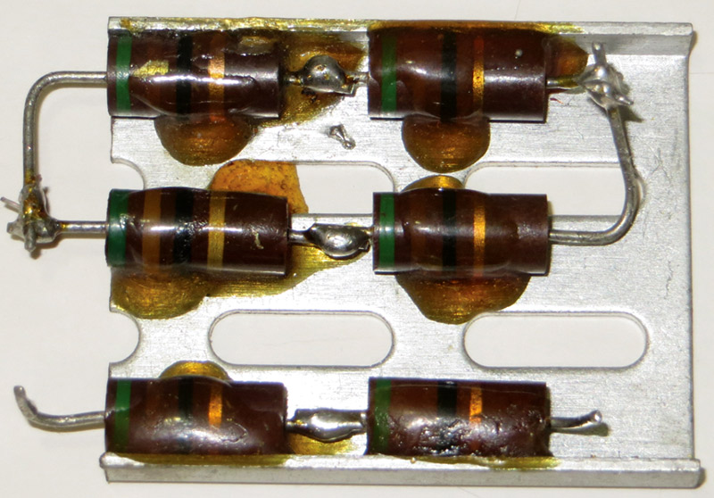
FIGURE 5. An array of one watt resistors on a heat spreader capable of dissipating 10 watts.
Depending on how they are connected together, I can get resistances of 10 ohms to 300 ohms. Two resistors in parallel have a resistance of 50/2 = 25 ohms — close enough to 24 ohms.
When this 25 ohm resistor was connected across the wall wart, the output voltage dropped considerably to 10.6V. Figure 6 shows the measured voltage response of the wall wart.
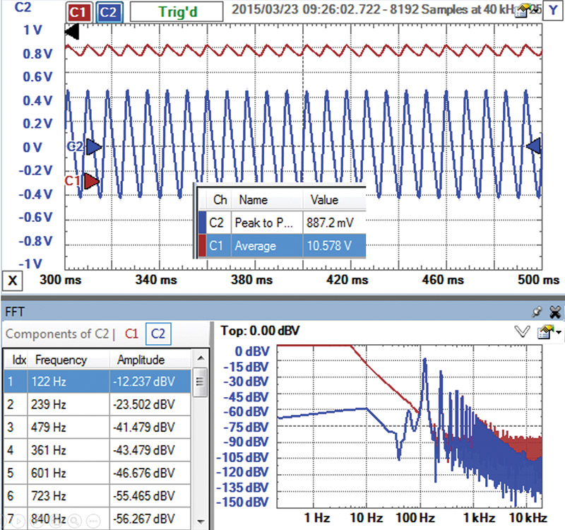
FIGURE 6. Measured DC and AC voltage response of the wall wart, nominally rated for 12V and 500 mA with a 25 ohm load. The performance is far from the rated spec.
The wall wart — with about 500 mA, its “rated” current — had a voltage of 10.6V with a peak-to-peak ripple of 0.89V. This is 8% peak-to-peak noise. Even though it was stamped 12V at 500 mA, its output voltage was only 10.6V with 8% peak-to-peak ripple noise. This gives you an idea of what to expect in some cases.
The Output Impedance of Power Supplies
The output voltage dropped from 13.6V unloaded to 10.6V with the 25 ohm resistor. All power sources will drop in output voltage when they supply current. This is due to their internal series resistance.
The simplest way of modeling the properties of a power supply is as an ideal DC voltage source with a series resistance. Figure 7 is the equivalent circuit model. In this model, as current flows out of the power supply, there is a voltage drop across the internal resistor. What we see is the output voltage after the IR drop across the resistor.
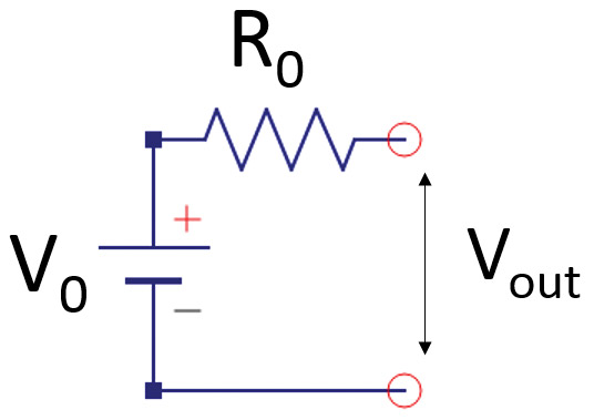
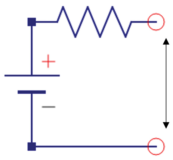
FIGURE 7. The equivalent circuit of all power sources showing the two important elements: an ideal DC voltage source and an internal series resistor.
There isn’t really a series resistor at the output of the power source; it just behaves this way. There is usually some other regulating circuitry like a bipolar transistor or MOSFET, or internal components which electrically look like a resistor. Knowing the value of the ideal DC source voltage and the equivalent internal resistance of the supply tells us the most important properties of the supply. Plus, they are easy to measure.
Use a Light Bulb as a Load Resistor
For future reference, if you need a 13 ohm high power resistor, a 75 watt incandescent light bulb will do. A 100 watt incandescent light bulb has a resistance of about 10 ohms. These are the resistances when cold. They increase as they get warmer. Of course, due to the internal electronics of a compact fluorescent light bulb (CFL), you can’t use one as a resistive load.
The DC voltage of the ideal source is just the voltage measured when the supply is unloaded. The output resistance can be calculated based on the voltage drop when connected to a known load. Figure 8 shows the equivalent circuit when the output is connected to a load resistor.
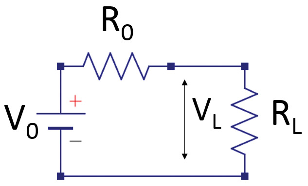
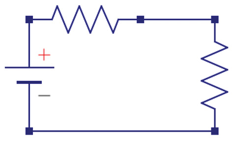
FIGURE 8. Equivalent circuit of the power source with an external load resistor.
With a little circuit analysis, the internal resistor, R0, can be calculated from the unloaded voltage, V0, the loaded voltage, VL, and the load resistor, RL, as:

To measure these features of any supply, just measure the voltage of the supply unloaded, then attach a known resistive load (watch out for smoke) and measure the voltage loaded. After a little arithmetic, you have the internal DC voltage and the internal resistive output.
The output voltage with any current load, IL, can then be calculated as:

For example, in this wall wart, the internal resistance is:

Its output voltage with any current load is:

Need a 12V source when it draws 500 mA? Don’t use this wall wart. In fact, when it draws more than 225 mA, the voltage will be below 12V. Unless you have characterized your wall wart, take the rating stamped on its outside only as a guideline — not a hard and fast performance spec.
While the internal DC voltage and the internal source resistor are really important, they are not the whole story. The other important term is the AC ripple noise when loaded down. These three terms are the most important to characterize the quality of a power source:
- Internal DC Voltage
- Internal Series Resistor
- Peak-to-peak AC Ripple when Loaded
Building an Arduino Based Automated Power Source Analyzer
Now that we know what to look for in a power source, we can automate the process of characterizing it and, along the way, test the quality of this simple equivalent circuit model. Just how well does a power source look like an ideal DC voltage and a series resistor?
Since I am enamored with the power of Arduinos, I decided to use one at the heart of my automated system. If I can change the current draw of the power source and measure the supply voltage as it draws current and the current load at the same time, I can plot the I-V curve. This should look like a straight line, with an intercept at the DC voltage and a slope equal to the internal resistor. From this curve, I can fit these two terms.
I used a simple transistor follower circuit as a resistive load. The input voltage to it will control the current. I wanted to ramp the current up so I could measure a few different values from 0 to a maximum. So, how do I get a ramp voltage from an Arduino?
Even though the specs for an Arduino say it has analog output, this is not quite correct. There are six digital pins — usually designated with a little squiggly line (“~”) next to them — which can be set up as pulse width modulated (PWM) signals. The duty cycle of a 500 Hz square wave is adjusted so the integrated value — or average value — can be changed.
However, to use these pins as an analog voltage — for example, to ramp up the voltage and the current load — would require a long integration time and they would still have some ripple on them.
I decided to use another approach to generate a ramp signal. I know I can get a precisely controlled digital output signal which is basically a square wave pulse. I could use a simple RC filter to turn the digital signal into a ramp. The output of the digital pin would charge up a capacitor through a resistor.
This voltage would then control the current through the transistor and the load on the power supply. Figure 9 shows this simple circuit.
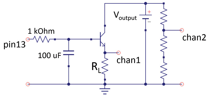
FIGURE 9. Transistor follower circuit with an RC integrator.
For this application, I used a 2N6040 — an NPN Darlington transistor. By adjusting the load resistor, RL, I can get any range of current I want. Given the limited number of time constants I wanted to wait and the forward drop through the transistor, the maximum voltage I would see across the resistor is about 3.5V. With a 10 ohm load resistor, the current will range from 0V to 3.5V/10 ohms = 350 mA.
I know I can set up an Arduino to sample the analog inputs every 10 msec. For about 50 measured points during the ramp-up, this is an on-time of about 0.5 sec. As long as the current is on for just one second every so often, I am not worried about the power consumption in the resistor.
For an on-time of 0.5 sec, I needed an RC time constant of about 0.1 seconds. With a 1K ohm series resistor, this means an integrating capacitor of about 0.1 sec/1000 ohms = 100 µF.
The voltage across the capacitor drives the base voltage, which then drives the current through the transistor. The voltage drop across the 10 ohm load resistor is a direct measure of the current through it.
Figure 10 shows an example of the input voltage from digital pin 13 and the resulting voltage across the 10 ohm load resistor.
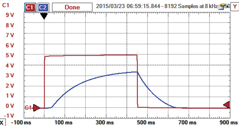
FIGURE 10. Voltage on pin 13 of the Arduino and the voltage across the 10 ohm load resistor — a measure of the current from the power source. The square signal is the voltage on pin 13 and the ramping signal is the voltage across the 10 ohm resistor.
This final system implemented with an Arduino Redboard from SparkFun ($19.95) and a small protoboard is shown in Figure 11.
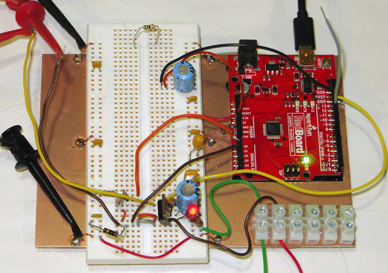
FIGURE 11. The final automated I-V system based on an Arduino with an integrating circuit and current load to a power source. The wires coming off from the bottom connect to the power supply to characterize.
Analyzing the I-V Curve in Excel
I wrote a simple sketch for the Arduino which sent a 0.5 sec digital pulse on pin 13 to drive current through the transistor from the power supply. I used two analog input pins to measure the voltage of the power supply and the current through it. Chan1 was a direct measure of the current from the supply, while chan2 was a scaled value of the supply output voltage.
Since many power sources are 15V or more, I used a voltage divider circuit to offer voltage drops from 1x, 0.5x, and 0.25x. This scaled the supply voltage to a range the analog input pin could handle. I use enough voltage drop to keep the maximum voltage on chan2 less than the 3.3V reference.
The sketch turns on pin 13, ramping the current from the power supply, and measures the supply current and the loaded voltage. These values are printed to the serial monitor.
I used PLX-DAQ to read the serial port and bring the data into a spreadsheet. The I-V data is plotted automatically as it comes in. I take the first five values to fit a linear trend line, and display the DC voltage and the slope which is the internal resistance. A steeper slope means a higher internal resistance.
When I click on the connect button in the PLX-DAQ control box, the Arduino is triggered to start the loop, the data is taken, printed to the serial port, read into Excel, and plotted — all automatically. Figure 12 is an example of the measured I-V curve for this wall wart.
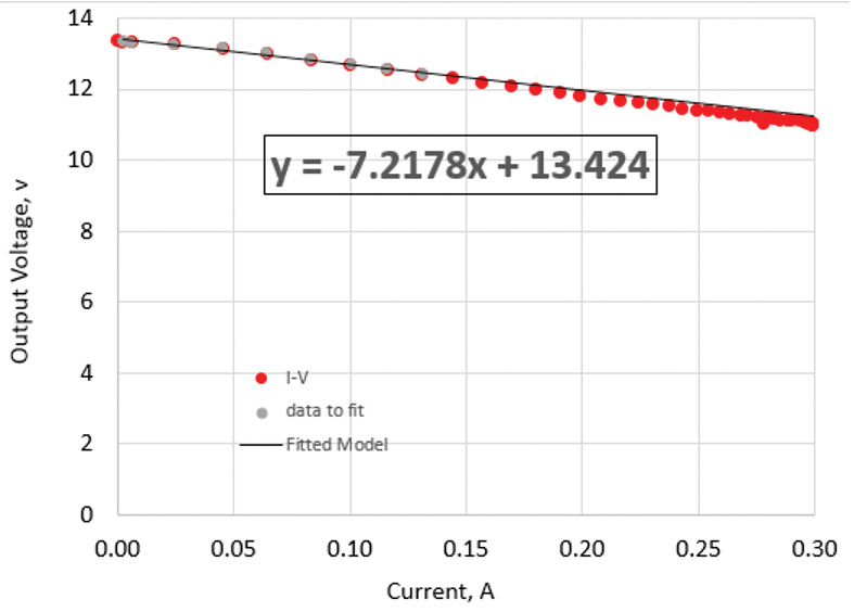
FIGURE 12. Measured I-V curve for the wall wart, showing the fitted values of the 13.4V open circuit load and 7.22 ohm output load impedance. This clearly shows how the output voltage of any power supply decreases with added current draw. The internal resistance is a good metric of how much voltage drop to expect.
We can see that the model for a constant internal resistance is a pretty good one. The 7.22 ohm internal resistance measured with this automated system is very close to the 7.1 ohm resistance I measured manually.
With this automated system, we can now explore the features of different power sources.
A Survey of Power Sources
Not all wall warts are created equal. I routinely use a 9V wall wart from SparkFun all the time. It is rated for 9V at 650 mA. Figure 13 shows the I-V curve and the AC ripple noise when loaded by 17 ohms, or drawing 530 mA.
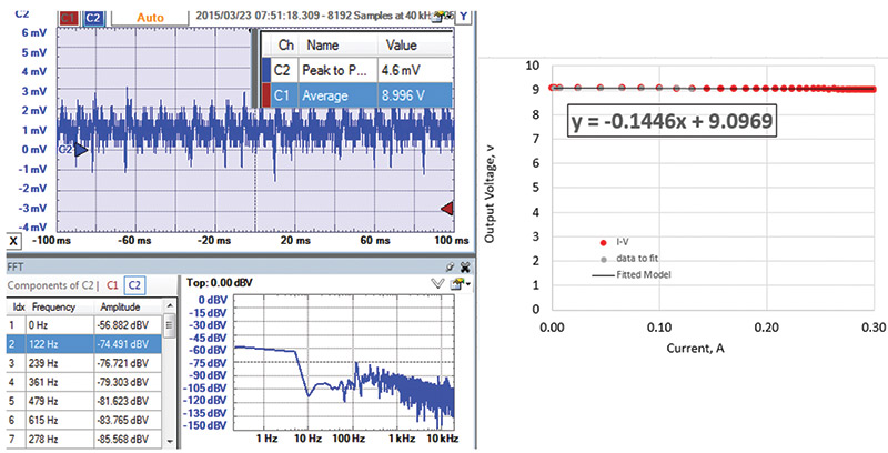
FIGURE 13. Characteristics of a 9V wall wart from SparkFun.
The peak-to-peak noise is remarkably low. The peak-to-peak voltage is 4.5 mV out of 9V, or less than 0.05% even loaded down. Its output impedance is 0.14 ohms.
The USB port is often used to supply current. The measured I-V curve and AC ripple with a 42 ohm load drawing 120 mA is shown in Figure 14.
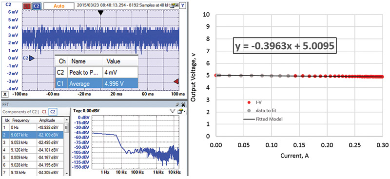
FIGURE 14. USB power performance.
It is a remarkably accurate 5V regulated supply with an output impedance of only 0.4 ohms. The AC ripple of the USB source I used was 4 mV peak-to-peak, with no discernable peak at 60 Hz or 120 Hz.
Sometimes one of the digital output pins of the Arduino is used to power a component. Figure 15 shows its I-V curve and AC ripple noise when set to HIGH.
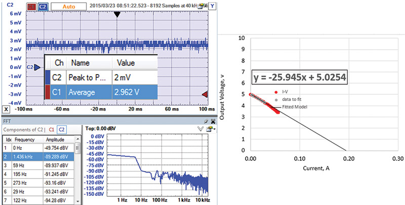
FIGURE 15. Arduino digital output pin as a power supply.
The output impedance of an Arduino pin is about 26 ohms. With a 40 ohm external resistor — or a total of 66 ohms — the current draw was 5V/66 ohms = 72 mA current. The ripple noise was about 2 mV peak-to-peak, but only a very small peak at 60 Hz. The voltage amplitude of the 60 Hz sine wave component is 10^(-89.3/20 )= 34 µV out of 5V.
Many portable applications use batteries as the power sources. Their properties vary a lot depending on the age of the battery and the type of battery. The AC ripple noise is typically at the noise floor of what the scope can measure. The amount of AC ripple noise from a battery is not really about the battery, but about how well it is shielded from external noise sources, and what it is connected to in its application.
I surveyed a number of 9V batteries and found the typical output impedance to be about 2.4 ohms. An example is shown in Figure 16.
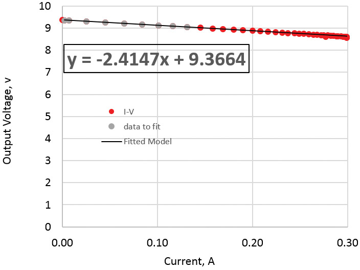
FIGURE 16. Measured output impedance of a 9V battery.
However, one battery — nominally also new — showed an output impedance of 8.5 ohms. This is just another example of the guideline: Buyer beware.
Two AAA batteries in series had an output resistance of 1.24 ohms. This implies the output impedance of one AAA battery would be about 0.62 ohms. Its IV curve is shown in Figure 17.
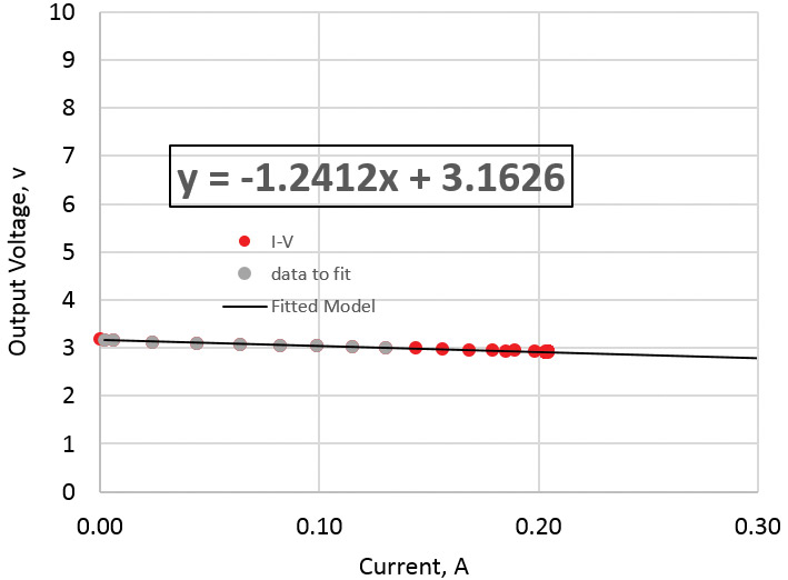
FIGURE 17. Measured output impedance of two AAA batteries in series.
Conclusion
Before you plug in that power source, try to answer four important questions:
- What is the current requirement for your application?
- Given the voltage you are going to use, what is the power dissipation you expect, and can you handle this?
- What is the unloaded output voltage and source resistance of the power source you plan to use, and what will be the loaded output voltage? Is this adequate?
- How much ripple noise is there on your power supply and is this okay in your applications?
With the simple measurement and analysis techniques offered here, you will be able to answer these questions and eliminate one common source of problems in your next project. NV
Avoid this Cross Talk Problem when You Use the ADC Pins
When any Arduino digital pins switch, they load the internal 5V rail on the die. This 5V supply is also used as the reference voltage for the ADC (analog-to-digital converter) pins. Figure A1 is an example of the measured voltage on pin 12, set as output HIGH, which is internally connected to the on-die 5V rail, while pin 13 is switched on.
We see the voltage noise on the on-die power rail drops as much as 20 mV when an output pin switches on. This results in noise on the reference voltage for the ADC and an artifact on the measured input voltage. This noise on the internal voltage rail will give false analog voltage readings to any of the ADC channels.
When I do precision voltage measurements, to get around this cross talk problem I use the 3.3V supply voltage on the Arduino board as the Vref for the analog pins. This gives a much cleaner and more stable analog voltage reading, but it also limits the highest voltage I can measure to be 3.3V.
In the sketch, you need to include the statement in the void setup() function, "analogReference(EXTERNAL);". This will connect the Vref of the ADC to the external Vref pin, which I connect to the 3.3V rail of the Redboard Arduino. I've measured this as a very clean signal.
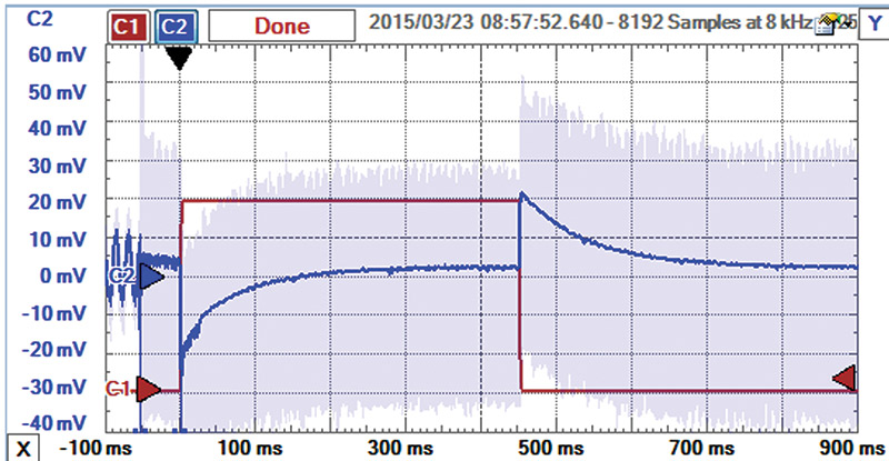
FIGURE A1. The measured voltage on pin 12 when pin 13 switches. The square signal is the voltage on pin 13 when it switched high. The signal that dips down then up is the voltage noise on pin 12, pegged HIGH. This is a direct measure of the voltage on the internal +5V rail which is also used as the Arduino's reference voltage for the ADC.
How Not to Generate Smoke
A resistor is really a component which is very efficient at turning electrical power into thermal power and getting hot. The power dissipation in a resistor can be estimated from:

If we measure voltage in volts, current in amps, and resistance in ohms, the power dissipated in the resistor is in watts. Resistor sizes are generally based on the power they can easily dissipate before getting too hot. Small physical size resistors have a small surface area and can't get rid of the heat fast enough before getting hot. Large body sizes have a large surface area and are more efficient at getting rid of the heat.
Large size axial lead resistors can easily dissipate one watt; the next smaller size is 1/2 watt, and the next smaller is 1/4 watt. The tiniest axial lead resistors are generally rated for only 1/8 watt. It's possible to get larger body size resistors rated for even higher power dissipation. Figure A2 shows examples of resistors with six different power ratings. It's all about their size.
Generally, if the power source is under 15V, to dissipate less than 1/2 watt and not worry about the power consumption requires a resistor greater than:

If you use a resistor less than about 500 ohms, be sure to put in the numbers to check if power will be a concern. If it is, watch out for smoke or engineer a solution that can adequately dissipate the power.
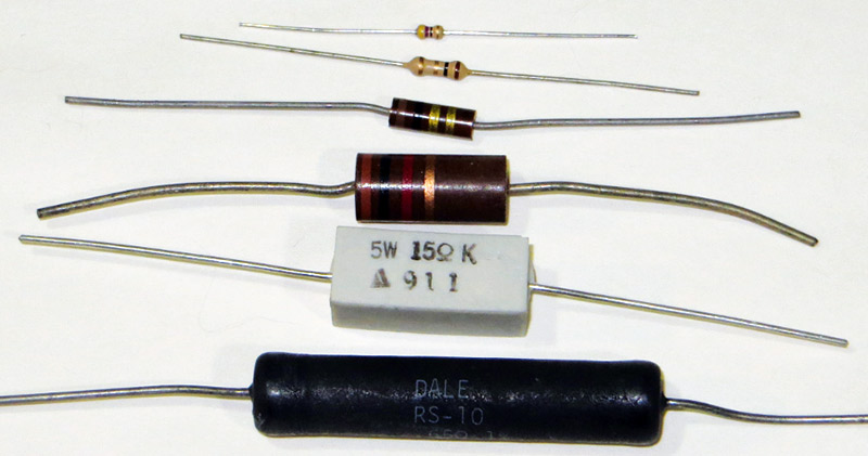
FIGURE A2. Resistors with six different power ratings: 10 watts, five watts, one watt, 1/2 watt, 1/4 watt, and 1/8 watt.
Choosing the Right Input Mode to a Scope
Most scopes have three input modes for a channel: 50 ohms, 1 megohm input, and AC coupled. The 50 ohm input is most useful when measuring signals in the 100 MHz and above bandwidth. It will terminate the coax cable connecting the scope to the device-under-test and prevent the artifact of reflections in the cable.
The 1 megohm input is the general-purpose setting to look at signals from DC to about 100 MHz, depending on the nature of the probe. The AC coupled input puts a 100 nF capacitor in series with the 1 megohm. This means DC signals are blocked. The time constant is about 0.1 sec (100 nF x 1 megohm), so signals above about 5 Hz are passed through to the receiver pretty much unchanged.
Resources
Digilent
Analog Discovery 100MS/s USB Oscilloscope & Logic Analyzer
Sparkfun Stuff
9V Power Supply
10K Thermistor
Mini Photocell
Arduino RedBoard
Dataq Instruments
Four-channel USB Data Acquisition Starter Kit
LabJack
USB Multifunction DAQ
Parallax
Parallax Data Acquisition tool (PLX-DAQ) software
Downloads
V-I_curvePlotter_B.ino, Excel File.