If you employ a wireless data or voice link, you use modes, too!
As you tune around the ham “bands” with a radio or spectrum analyzer, you can hear and see an awful lot of different signal types. Some are whistles, some are warbles or chirps, some sound like vacuum cleaners, and some even sound like voices if you have the right receiver. These different signals are called “modes” by hams — each with its own purpose, strengths, and weaknesses. This article is an overview of fundamental modes used in communication systems. Next time, we’ll cover more advanced modes used for data transmission.
RF Signal Basics
All signals — RF or not — are built out of sine waves (even digital signals — a topic for another time). A sine wave has an amplitude and a frequency. Amplitude is the “size” of the sine wave, and frequency is the number of complete cycles (from zero to maximum to zero to minimum and back to zero) every second, measured in Hertz (Hz). The time it takes for one cycle is the signal’s period (T), measured in units of time — such as nanoseconds for signals in the GHz range.
Each cycle of the sine wave is divided into 360 degrees — just like the circle. (Radians are another type of angular measurement and a full cycle of a sine wave contains 2π radians.) The position within the cycle is called phase, measured in degrees or radians as shown in Figure 1A. If two sine waves have the same frequency and begin their cycles at the same time, the signals are in-phase. If those same signals begin their cycles at different times, they have a phase difference or phase shift (Figure 1B). If the time difference is one-half cycle so that both signals are zero at the same time but changing in opposite directions, they are out-of-phase or anti-phase (Figure 1C).
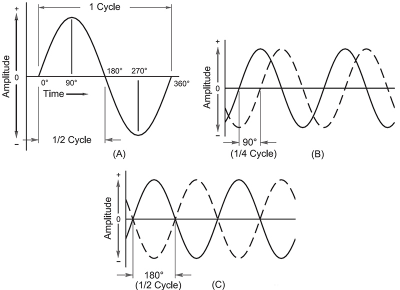
FIGURE 1. Phase is used as a measure of time within the signal. Each cycle of a sine wave is divided into 360 degrees of phase (A). Parts (B) and (C) show two special cases. In (B), the two signals are 90 degrees out of phase, and in (C) they are 180 degrees out of phase or anti-phase. (Graphic courtesy of the American Radio Relay League.)
Phase or Polarity?
It is important to distinguish between phase, which represents time or position in a waveform, and polarity, meaning the convention of positive and negative voltage or current. It is quite possible for two signals to have opposite polarities but still be “in phase,” for example. Phase in an AC power system refers to one of the distinct voltage waveforms generated by the utility.
Sine waves are generally considered to be RF or radio frequency signals if the wave’s frequency is higher than the audio range, which has a maximum frequency of 20-30 kHz. (Some special-purpose communication systems communicate with radio signals at lower frequencies.) The RF spectrum is very broad, extending from just above the audio range to hundreds of GHz. Most wireless systems used by hobbyists range from about 1 MHz to around 10 GHz.
Carrying Information with an RF Signal
By itself, a continuous sine wave doesn’t carry any useful information. It’s just “there.” However, if we vary one of the sine wave characteristics — its amplitude, frequency, or phase — we can use those variations to encode information. This is called modulation. Because it’s hard to transmit audio or data signals any useful distance by themselves, modulation is used to add them to the RF signal which can be easily transmitted over great distances. When the signal is received, another process can recover the information by decoding the RF signal variations. This is called demodulation. (This is where the term modem comes from — modulation-demodulation.)
Because the difference between the information and RF signal frequencies is so great (usually several orders of magnitude), viewing the modulated RF signal on an oscilloscope gives an incomplete picture. To help visualize what happens to an RF signal when it is modulated, engineers display the signal in the frequency domain as in Figure 2. Amplitude is still on the vertical axis, but now the horizontal axis shows frequency. This is what you would see on a spectrum analyzer display. Tuning a receiver can be imagined as sliding its receive window back and forth along the horizontal axis. The receiver will hear and attempt to demodulate any signal in the window.
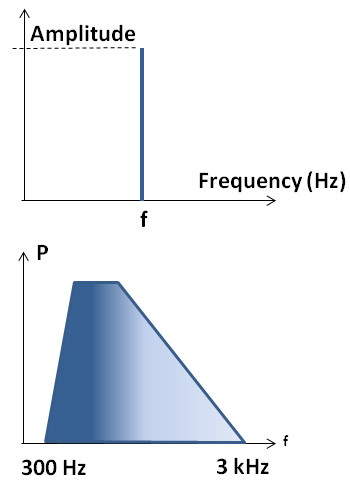
FIGURE 2. The spectrum of a single sine wave (A) has only one component, shown as a vertical line at one frequency (f) and with a fixed amplitude. The spectrum of a typical speech waveform (B) consists of many component signals with different frequencies and amplitudes. Most communication systems consider speech to extend from 300 to 3,000 Hz.
That steady sine wave can be represented as a single vertical line as in Figure 2A — this unmodulated signal has a single frequency (f) and a constant amplitude. The information to be added to a signal generally has a more complicated spectrum.
For example, the spectrum in Figure 2B is typical of human speech: many individual frequency components ranging from strong ones with higher amplitudes around 300 Hz, then tapering off around 3 kHz. We could draw a vertical line as in Figure 2A for every different component in a speech signal, but it is a lot easier to draw a shape that represents the spectrum of speech. Different types of information (data, music, speech, telephone dialing tones, etc.) have spectra with different shapes.
Modes = Information + Modulation + Protocol
It is not enough to simply add information onto an RF signal and transmit it. The receiving station (even a little Arduino wireless data shield can be considered a “station”) has to know what frequency range to listen on, what kind of modulation is being used, the type of information being sent, and how it is encoded. This defines the air link which defines the signal you would observe on the air.
Once the air link characteristics are determined, the receiver also has to understand the protocol being used — the “rules of engagement” for establishing contact (a session in datacomm-speak) and managing the flow of information. Finally, the receiver has to be set up to recover the information and present it to the user in an appropriate format. It wouldn’t do for a receiver to recover 1s and 0s representing an MP3 file but send them to the speaker as a series of pops and clicks!
All three parts — the type of information being transferred, the air link that gets the information from point A to point B, and the protocol that manages the transfer — create what hams call a mode and what the FCC (Federal Communications Commission) refers to as an emission.
For example, if I want to send a text file via ham radio using the Winlink system (www.winlink.org — pretty cool, huh?) on the shortwave bands, I would use a mode consisting of the PACTOR protocol and AFSK (audio frequency-shift keying) to modulate my voice transmitter. Text characters + PACTOR + AFSK form one of the many permitted modes used by amateurs.
In my living room, I might use a different mode consisting of digitized audio + Bluetooth which specifies GMSK modulation to stream music to my wireless headphones.
Hopefully, you now get the idea of combining data with a protocol with a way of modulating an RF signal. Let’s take a look at the modes used by hams.
FCC Emission Designators
In order to write precise rules for users of the RF spectrum, the FCC has to use equally precise definitions of what those signals are. Those definitions are called emission designators. Each designator consists of a sequence of characters that define bandwidth, modulation, nature of the signal, and the type of information. For example, AM broadcast signals with the full 10 kHz audio bandwidth have the designator 20K00A3EGN. You can find out all you ever wanted to know about emission designators in this guide. There are an amazing number of signal types “out there!”
On-Off Keying (OOK) or “CW”
The very oldest mode of wireless transmission is the simplest, consisting of just turning a transmitter on and off in a coded pattern that represents characters. (Turning a transmitter on is called “keying” whether a telegraph key is used or not.) The coded pattern used by nearly all hams is Morse code and it has been around since 1840 in several varieties (en.wikipedia.org/wiki/Morse_code). The first was American Morse, then the Continental Code was created. Finally, today’s International Morse was defined by the ITU and is still in use today — it’s actually quite popular (see the companion article in this issue by John Thompson on CW making a comeback).
What does “CW” — standing for the old term “continuous wave” used for Morse code transmissions such as in Figure 3 — “look like” to a spectrum analyzer or a tunable receiver? Going back to Figure 2A, you would “see” a vertical line appearing and disappearing in the pattern of Morse code. The characteristic “beeping” comes from circuitry in a CW receiver that converts the presence of the signal into an audio tone. No signal, no tone. It’s very simple and easy to learn.
Amplitude Modulation or AM
The next oldest mode is amplitude modulation or AM. (Hams sometimes jokingly call AM “ancient modulation.”) OOK is a simple form of AM in which the amplitude is either zero or non-zero, but to send speech or music something more capable is required. The simplest way of creating an AM signal is to first create an unmodulated RF signal called a carrier. Next, make its amplitude larger and smaller in the same way a speech waveform gets louder and quieter.
Figure 3 shows the result if a single audio tone is used as the modulating signal. The resulting AM signal can be transmitted over the air and any receiver that can follow the signal’s outline — called the envelope — can reproduce the original speech or music. It’s surprisingly easy.
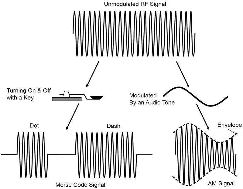
FIGURE 3. On-Off Keying (OOK) of an unmodulated carrier signal in a pattern such as Morse code is a very simple form of amplitude modulation (AM). A tone or speech can also be used to modulate the signal, resulting in a signal whose shape or envelope contains the information from the tone or speech. (Graphic courtesy of the American Radio Relay League.)
On our spectrum analyzer display, however, the simple vertical line of the original RF signal has suddenly become quite a bit more complicated. The AM signal now consists of the steady RF carrier flanked by symmetrical signals on either side (called sidebands) as shown in Figure 4. This combination of a carrier and sidebands is called a composite signal — one with several components.
Figure 4A shows what happens for modulation by a single tone. A sideband is created above (the upper sideband or USB) and below (the lower sideband or LSB) the carrier. The frequency of the sideband differs from the carrier by the frequency of the tone. If the tone is a 1,000 Hz tone and the carrier’s frequency is 1 MHz, the sidebands would be found at 1.001 and 0.999 MHz.
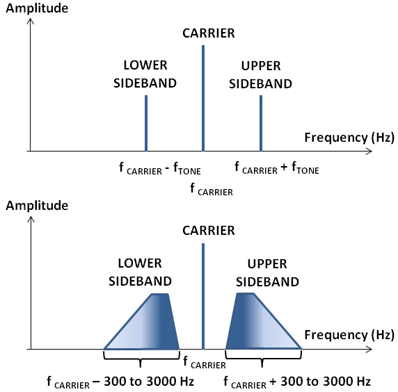
FIGURE 4. The spectrum of an AM signal modulated by a single tone (A) shows the carrier and two sidebands, separated from the carrier by the frequency of the modulating tone. The spectrum of an AM signal modulated by complex information such as speech is shown at (B).
If speech was used to modulate the carrier, the situation of Figure 4B would result. The speech would be translated into sidebands with the same bandwidth as the speech itself: one above and one below the carrier. What’s particularly important to note is the sidebands are mirror images of each other. The USB still has low speech components below the higher components, but the LSB is inverted. In both cases, the individual speech components are symmetric about the carrier.
Single Sideband or SSB
Why does AM need two sidebands with the speech information? What does the carrier do? The answers are “it doesn’t” and “nothing!” AM is easy to generate and receivers are simple, but the cost is low efficiency. Fully one-half of an AM signal’s power remains in the carrier, which actually carries no information. The modulating information is duplicated in the sidebands, as well. Only one-fourth of the AM signal’s power goes into a unique signal — one of the sidebands.
That Warm AM Sound
AM broadcast signals were once the highest of hi-fi, and many homes sported a large console tube-type receiver with large speakers. Ball games, musical programs, and live announcers really do sound great on this equipment! Many amateurs enjoy keeping their “big iron” rigs on the air for the warmth of the AM audio with its better bass response and relaxed style of operating. AM will be around a long time — both broadcast and ham.
During the 1930s, research showed that there were several ways of removing or suppressing the carrier and one of the sidebands. Either of the remaining sidebands carried all of the information, but the receiver had to supply the missing carrier — which turns out to provide a frequency and phase reference for demodulating the sideband.
Advances in receiver design during and after WWII made SSB practical, and it soon replaced AM for most point-to-point communication uses. By putting all of the power into one sideband, the effect on the signal-to-noise ratio (SNR) was a four-fold (or 6 dB) improvement. Either smaller transmitters could be used for equivalent range or the same power could double the signal’s range.
Either LSB or USB can be used, and both are common today in amateur radio, marine radio, aviation, and government communications. Because of the mirror image sidebands, the receiver has to be set to receive the correct sideband — LSB or USB — or the demodulated information will be garbled. Certain transceiver design choices made decades ago led to the convention of using LSB below and USB above 9 MHz, but functionally they are equivalent.
Frequency Modulation (FM) and Phase Modulation (PM)
Like amplitude, both frequency and phase can be modulated to add information to an RF carrier signal. FM or PM is created by varying the value of a resonant circuit’s capacitor (FM) or the reactance of a phase-shifting capacitor (PM). Frequency and phase are closely related mathematically and so are FM and PM. An unmodulated RF sine wave is described by A sin (φ, where the sine wave’s amplitude is A and its angle is φ = 2 πft. AM varies A, and both FM and PM vary φ. As a result, FM and PM are called angle modulation.
Changing a signal’s frequency or phase is equivalent so FM and PM are almost the same. The main difference between FM and PM is that phase modulation accentuates the higher frequencies of the modulating signals — an effect called pre-emphasis — as if a high-pass filter was acting on the audio. To restore a “flat” frequency response, complementary de-emphasis networks (a low-pass filter) had to be used in the receiver.
The spectrum of FM/PM signals is much more complex than AM and SSB signals. (I’ll just use FM to refer to both FM and PM from here on.) As with AM, there is a single carrier signal. However, to create a signal with a frequency (or phase) that varies with a modulating signal, essentially an infinite number of sidebands are required! (The mathematical expression that defines the spectrum is called a Bessel function.) The amplitudes of the carrier and all the sideband components are controlled by the modulating signal’s amplitude which determines the signal’s modulation index.
Figure 5 shows FM signals modulated by a single tone at different modulation indexes. You can see bandwidth increasing with the modulation index. The power in an FM signal is divided up between the carrier and all of the sidebands so that the total power is always the same — FM is a constant power signal. When an FM transmitter is keyed, the output power is the same whether you are speaking or not. Note that for some values of the modulation index (such as 2.4), the carrier can even be zero.
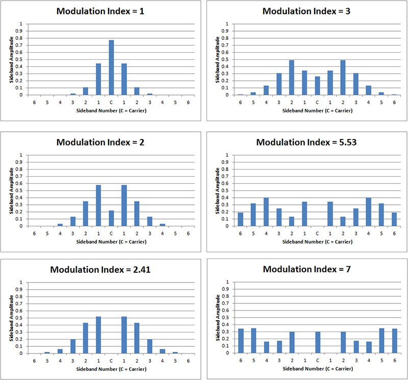
FIGURE 5. The spectrum of FM signals is very complex, depending on both the modulating signal's frequency and amplitude which control the signal's modulation index. At some values for the index (such as 2.4), the carrier disappears. There are an infinite number of sidebands, but the FM signal's power is constant.
Narrowband FM (NBFM) signals have a modulation index less than or equal to one. It is used where power efficiency is more important than fidelity, such as for handheld FM transceivers. Wideband FM (WBFM) signals — such as for high-fidelity commercial FM broadcast — have a modulation index of 10 or more, and occupy up to 150 kHz of bandwidth.
Why go to all the trouble of FM and PM and those complicated signals? Originally, all voice-carrying radio signals were AM. As anyone who has listened to AM radio knows, static can be a real problem. It’s an AM signal just like the one you’re trying to listen to, so the radio “demodulates” its crashes and buzzes, too. An FM receiver, though, only responds to variations in signal frequency, not amplitude. So, it can almost completely reject AM static and noise. As a result, a strong FM signal has almost no noise — even in the middle of stormy weather.
As an additional benefit, FM’s constant power nature means that amplifiers for the RF signal don’t have to be linear so they can reproduce the signal’s envelope. That means the amplifiers are simpler, require far fewer adjustments, and can be much more efficient than linear amplifiers for AM or SSB signals.
Data Signals Next Time
If you want more information about AM, FM, and SSB, check the ARRL’s Radio Technology Portal’s (www.arrl.org/tech-portal) Radio Technology Topics section. The Agilent company has also published a detailed application note about spectrum analysis of AM and FM as well, that’s available here. There’s more than enough to keep you busy until the next article comes along!
While digital data can be sent over AM or FM systems, it’s more effective to use modes designed specifically for data. In a future Ham’s Wireless Workbench, we’ll start with a simple two-tone frequency-shift keying (FSK) signal and work our way up! NV