This article uses simulation to explore harmonics, which are whole number multiples of a base frequency. Harmonics form a base line for testing, comparing, and explaining various circuits. The term can also refer to the ratio of the frequency of such a signal or wave to the frequency of the reference signal or wave.
To start off, I simulated a base square wave with a sine wave harmonic at twice the base frequency as in Figure 1.
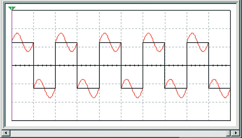
FIGURE 1. Enhanced square wave with second harmonic interference.
I put a square wave source in series with a sine wave source at twice the square wave's frequency and viewed the result with a virtual dual trace oscilloscope. The base frequency is in black and the sine wave is in red.
Figure 2 shows the simulated circuit used to create the wave form in Figure 1.
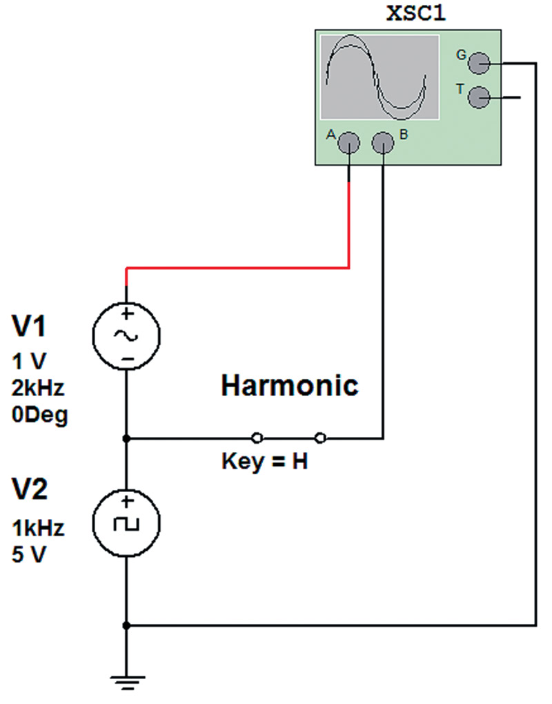
FIGURE 2. Simulation circuit used in Figure 1.
A harmonic switch was added so that the enhancement could be switched off and the base frequency waveform viewed. The operation of the harmonic switch is demonstrated in Figure 3.
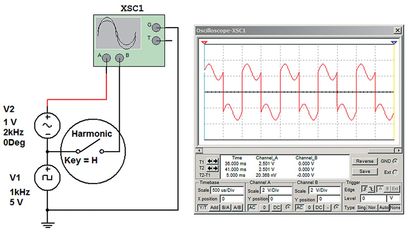
FIGURE 3. Circuit with harmonic enhancement switched off.
Using the circuit in Figure 2, we can shift the amplitude, phase, and frequency of the harmonic. There are some key points to be made here. Harmonics produce variations in the shape of the base wave. The higher the amplitude of the harmonic frequency, the greater the change in the base wave’s shape. The higher the multiple the harmonic frequency is, the greater the number of changes that occur to each base wave cycle. These concepts are demonstrated in Figure 4.
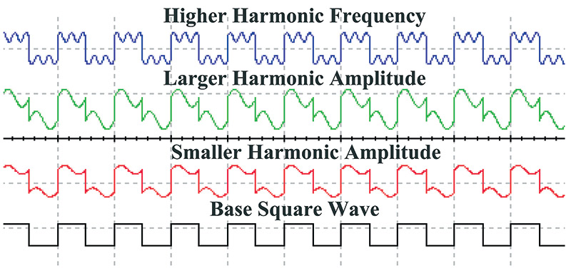
FIGURE 4. The effect of harmonics on base signals.
In Figure 5, I took one of the signals in Figure 4 and (using Microsoft Paint) shifted the position of the traces so as to recreate the harmonic signal. Below that, I compared one cycle to another by overlapping the signals.
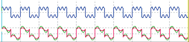
FIGURE 5. Signal graphic manipulation.
Let’s look a little more deeply at harmonics. The thing that is significant about harmonics is that they are stable, repeating every cycle. If I shift the harmonic in Figure 2 by 300 Hz, you will see that the red signal shifts in phase between cycles of the square wave. Figure 5 shows a square wave with a non-harmonic signal at near twice the base frequency.
Visualizing the frequency content of a waveform is challenging. This is most true with live signals with their constant small changes. If possible, store the trace and look back at it in a stationary form. Focus in on the characteristics of the waveform that are stable, keeping in mind how the base waveform looked. Figure 6 shows the original base waveform placed on top of the harmonic signal to highlight the differences.
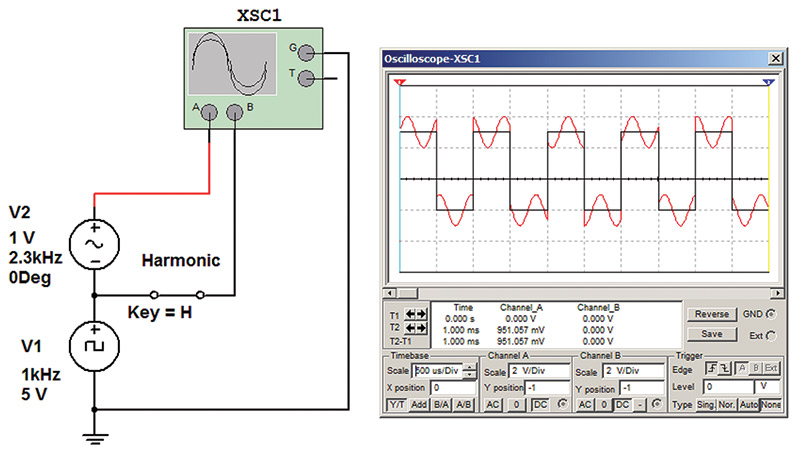
FIGURE 6. Square wave with non-harmonic interference highlighted in red.
You are looking for variations in the signal that repeat from cycle to cycle, not just random changes in the signal. Figure 7 is an illustration of a square wave with non-harmonic interference. Note the variation in the change between cycles.

FIGURE 7. Square wave with non-harmonic interference.
The differentiation between harmonic and non-harmonic interference is important. Harmonics are caused by non-linear changes in current and voltage. Harmonic interference is commonly the result of a distortion to the base signal, such as clipping with a diode. Non-harmonic interference is from a source unrelated to the base signal.
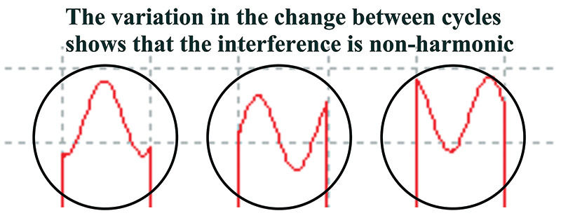
FIGURE 8. Interpreting non-harmonic interference.
Next, let’s try to identify specific harmonic frequencies. The closest we can get to this with our technique is to identify the harmonic number. The harmonic number is the multiple of the base frequency that the harmonic frequency equals. For example, if the base frequency was 1,000 Hz, the third harmonic would be 3,000 Hz.
This technique is not good for harmonics alone. It can also be used to identify near-harmonic interference. This is in many cases as accurate as necessary, for example, when selecting a filter. Make note of the number of changes that occur within a waveform cycle and the shifting position of the changes. This is easiest when you’re able to observe several cycles at once.
To help visualize this, I simulated a square wave harmonic on a sine wave base frequency. This caused the harmonic to produce a definitive red pulse on the base sine wave. In Figure 9, I generated a sine wave with a square wave set at the fifth harmonic.
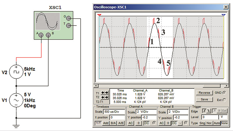
FIGURE 9. Sine wave with a square wave at the fifth harmonic.
The number of the harmonic corresponds with the number of times the change occurs in a cycle. In this case, the change that occurred was five red pulses that appeared in each full cycle of the sine wave.
When I went to school, I was taught that a square wave consisted of a fundamental frequency and all its odd harmonics. If we virtually reverse-engineer a square wave and reassemble it from its harmonics, we will see that this is not entirely true. As shown in Figure 10, when attempting to add a fundamental frequency and its odd harmonics, nothing approximating a square wave results because the harmonic formula is incorrect.
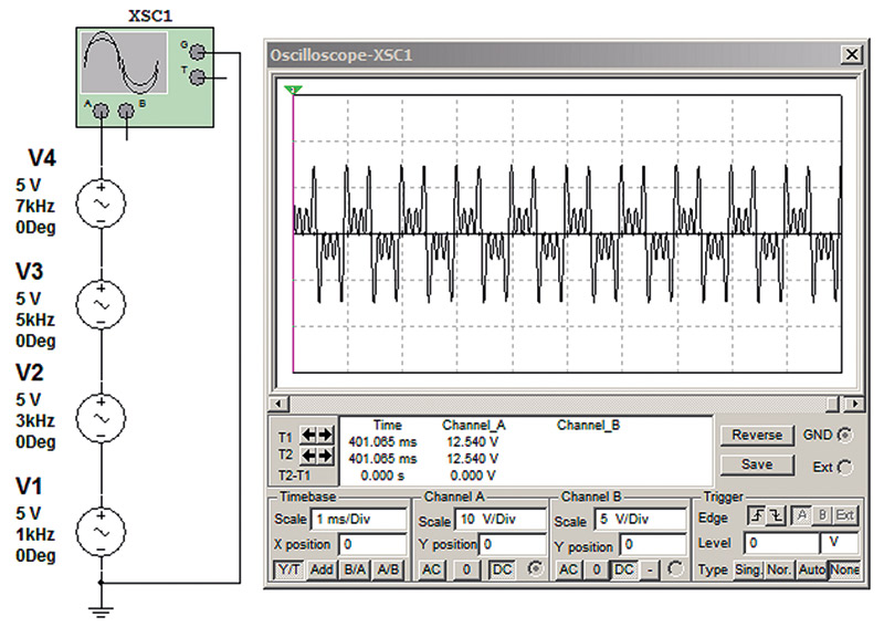
FIGURE 10. Signal produced by equal level odd harmonics.
In a square wave, the level of each harmonic should equal the base amplitude divided by the harmonic number. Observe how Figure 11 more closely approximates a square wave.
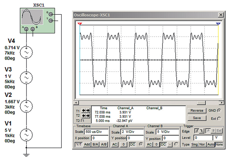
FIGURE 11. Waveform with harmonic levels adjusted to approximate a square wave.
Both triangle and square waves contain the same harmonics; it is only the harmonic mix that is different. Triangle waves contain less energy in their harmonics, and as a result more closely resemble a sine wave (as illustrated in Figure 12).
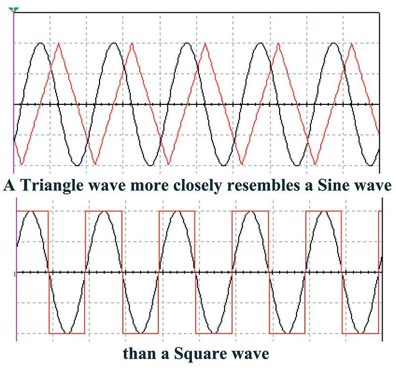
FIGURE 12. Triangle waves more closely resemble sine waves.
It is often not the frequency of a harmonic that matters, but the energy contained in the harmonics that could possibly result in interference. The magnitude of the change to a sine wave is an indication of the energy contained in the harmonics. By noting the differences between a signal and a sine wave, one can start to gauge the energy in the harmonics.
In a square wave, the amplitude of the harmonics is determined by dividing the amplitude of the base frequency by the harmonic number. In a triangle wave, the amplitude of the harmonics is determined by dividing the amplitude of the frequency by the square of the harmonic number. Figure 13 shows a dual trace of a square wave and triangle wave overlapping. The red square wave contains more energy in its harmonics. The rapid change of signal level and the flat regions in the square wave are indicative of higher energy levels in the harmonics.
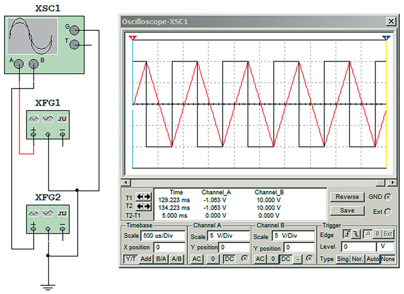
FIGURE 13. Triangle and square waves.
This information can form a base line for testing filter circuits. In Figure 14, a square wave was sent through both a high pass and a low pass filter. The high pass filter blocked the base frequency while passing the higher harmonics; this produced spiking or rapid changes in levels which is indicative of high frequencies. The low pass filter passing the base frequency while blocking the higher harmonics produced a waveform resembling a sine or triangle wave, which is indicative of lower energy in the harmonics.
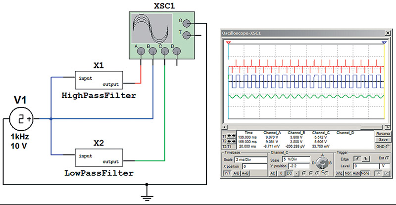
FIGURE 14. Square wave filtering.
The comparison of the output of a known good filter to the one under test can provide valuable information. If known, select a square wave frequency in the range of the filter circuit, or otherwise just adjust the square wave frequency until you see a significant change in the filter output.
When using a building block approach to produce a square wave, it is impossible to supply every harmonic. So, the question is how many harmonics are adequate. The answer is the more harmonics used, the faster the square wave will change levels, and the longer the flat areas will be on the top and bottom.
Figure 15 shows a signal made of just the first and third harmonic in black compared to a real square in red. You can see the flat areas of the square wave are larger and the time it takes for the square wave to change levels is faster. The good square wave is indicated by the reduction in rise and fall times and the longer flat regions.
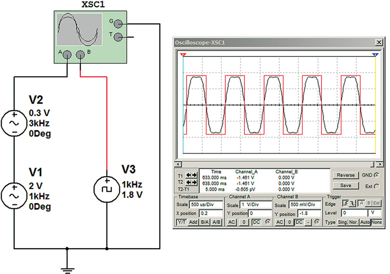
FIGURE 15. Limited harmonic simulated square wave.
Square waves can be used to evaluate sound systems. In Figure 16, a square wave was input into a simulated speaker where the impact was captured on an oscilloscope.
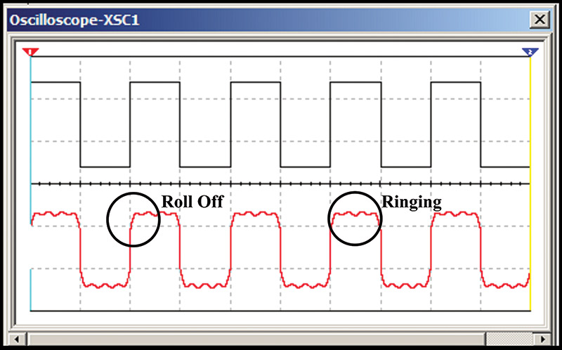
FIGURE 16. Roll off and ringing.
This technique can be used to detect high and low frequency roll-off, as well as over-shoot and ringing. If you are heavily into sound engineering and want to use this process to evaluate systems, you will need a high bandwidth square wave in order to capture all the harmonic information. This combined with the FFT (Fast Fourier Transform) feature now available on many oscilloscopes offers a great tool for the comparison of sound systems.
Final Thoughts
With simulation programs and a building block approach, you can systematically look at the structure of complex signals. The building block approach allows for the testing of electronic circuits under very controlled conditions. This technique also enables precise control of signal bandwidth and spectral content.
The building block approach can be used to produce a variety of complex wave forms including AM and SSB. It can be used to inject noise into a signal and test the performance of various types of detectors.
These simulation techniques can be looked at by the technician and the technical educator as tools for testing, comparing, and explaining various circuits. NV
