A logic analyzer — like so many electronic test and measurement tools — provides a solution to a particular class of problems. These include digital hardware debugging, design verification, and embedded software debugging. A logic analyzer is an indispensable tool if you design and troubleshoot digital circuits.
Logic analyzers simultaneously measure numerous digital signals with challenging trigger requirements. If you are using new devices, you’ll soon discover that debugging microprocessor-based designs requires more inputs than oscilloscopes can offer. Logic analyzers — with their multiple inputs — solve these problems. These instruments have steadily increased, both in their acquisition rates and channel counts, keeping pace with advancing digital technology.
There are similarities and differences between oscilloscopes and logic analyzers. To better understand how the two instruments address their respective applications, let’s compare their individual capabilities. After triggering on a complicated sequence of digital events, a logic analyzer can copy large amounts of digital data from the SUT (system under test.) Advanced logic analyzers behave like software debuggers that trace computer programs' flow.
HISTORY OF LOGIC ANALYZERS
The first logic analyzer appeared in 1967 as HP engineer Gary Gordon’s personal “bench project.” Just six years earlier, Gary became a company hero as an intern in the oscilloscope lab by solving their digital sampling scopes drifting problem when the time base changed.
Gordon’s involvement with digital oscilloscopes before inventing the logic analyzer is not surprising since logical analyzers evolved from DSOs. Logic analyzers evolved almost simultaneously with the first commercially available microprocessors. The first logic analyzers emphasized operations closely akin to oscilloscopes for hardware debugging and test, later becoming more concerned with monitoring microprocessor signal activity and software debugging.
A DSO (digital storage oscilloscope) or any oscilloscope is an instrument that primarily reveals the signal’s amplitude, rise time, and other analog characteristics, such as phase relationships, peaks, time between adjacent edges, etc. (see Figure 1). A scope’s vertical axis represents voltage and its horizontal axis represents time.
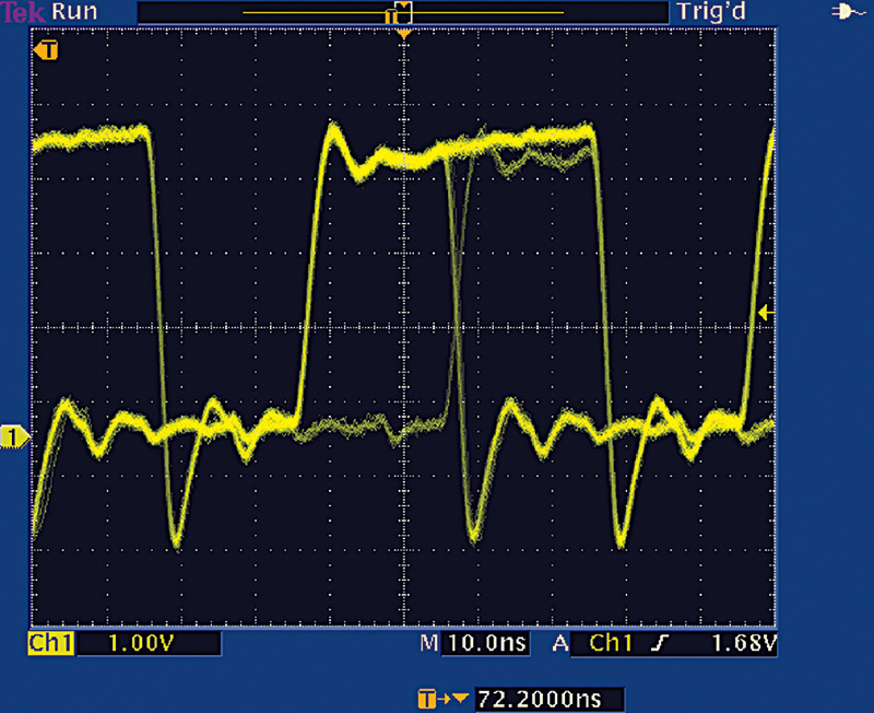
FIGURE 1. An oscilloscope’s display reveals signal details of a largely analog nature, such as rise and fall times, amplitude, and other subtle characteristics.
What a Logic Analyzer Does
A logic analyzer solely measures digital, not analog signals! It can capture many digital signals simultaneously and display their often complex timing relationship to one another. However, some logic analyzers slightly transgress into the scope’s domain by detecting glitches and setup and hold timing violations. But mainly, logic analyzers debug elusive, intermittent signals, with some advanced ones even correlating source code with specific hardware problems.
More on the Digital Oscilloscope
The DSO is for general-purpose signal viewing. Its sample rate (up to 20 Gs/sec) and bandwidth enable it to capture many data points over a short span. This allows measurements of signal transitions (edges), transient events, and small time increments. While DSOs can view the same digital signals as a logic analyzer, most DSO users concentrate on analog measurements such as rise- and fall-times, peak amplitudes and the elapsed time between edges. Figure 1 illustrates the oscilloscope’s strengths. The waveform (though taken from a digital circuit) reveals the analog characteristics of the signal, all of which can have an effect on the signal’s ability to perform its function. Ringing, overshoot, roll off in the rising edge, and other aberrations appearing periodically exist here.
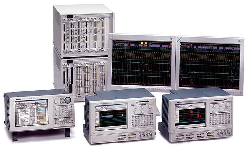
With a modem oscilloscope’s built-in tools such as cursors and automated measurements, it’s easy to verify signal integrity problems impacting your design. Purely analog signals — such as the output of a microphone or digital-to-analog converter — can only be monitored with an instrument that records analog details (see Figure 2).
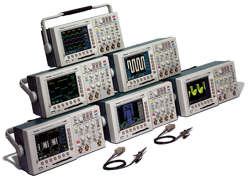
FIGURE 2. A family of modern high performance Tektronix DSOs.
Logic Analyzer Details
The most obvious difference between these two instruments is the number of channels (inputs). Typical digital oscilloscopes have up to four signal inputs. Logic analyzers have between 34 and 136 channels. Each accepts one digital signal. Some complex system designs require thousands of input channels. Appropriately scaled logic analyzers are available for those tasks, as well.
A logic analyzer detects logic threshold levels (see Figure 3).
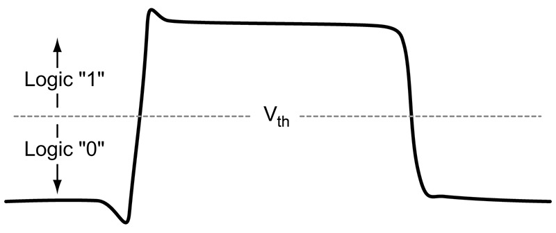
FIGURE 3. The logic analyzer reveals a more limited picture of a signal’s characteristics — just logic levels relative to a threshold voltage level.
When the input is above the threshold voltage, the level is said to be “high” or “1;” conversely, the level below the threshold voltage is a “low” or “0.” When a logic analyzer samples an input, it stores a 1 or a 0, depending on the level of the signal relative to the voltage threshold.
A logic analyzer’s waveform timing display is similar to that of a timing diagram found in a data sheet or produced by a simulator. All of the signals are time-correlated and effectively show progressive system “snapshots” through time.
A logic analyzer’s digital design verification and debugging features — such as sophisticated triggering — allow you to specify the conditions under which the logic analyzer acquires data. High-density probes and adapters simplify connecting to the SUT. Analysis capabilities translate captured data into processor instructions and correlate it to source code.
When to Use a Logic Analyzer vs. a DSO
A DSO is an ideal test instrument when you need to measure:
- A few analog characteristics of no more than four signals at a time.
- You need to know analog characteristics of a signal, such as rise and fall times, phase, power, current, amplitude, and edge relationships.
- You need to determine a signal’s stability (jitter).
- You need to measure timing margins such as setup/hold and propagation delays.
- You need to determine transient states, such as runt signals, glitches, and metastable states.
A logic analyzer is best when you need to:
- Debug and verify digital system operations.
- Trace and correlate many digital signals simultaneously.
- Detect and analyze timing relationships for many digital signals.
- Trace embedded software operations.
Logic Analyzer Architecture and Operation
There are four steps to using a logic analyzer:
- Probe (connect to the SUT)
- Setup (clock mode and triggering)
- Acquire
- Analyze and display
Each block in the simple logic analyzer block diagram shown in Figure 4 symbolizes several hardware and/or software elements.
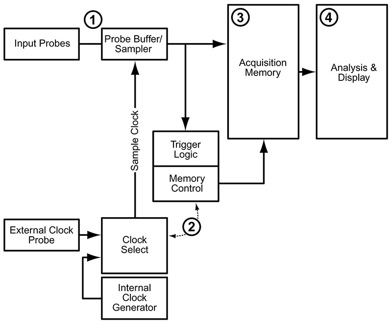
FIGURE 4. A greatly simplified functional block diagram of a logic analyzer.
The block numbers correspond to the four steps just listed. The acquisition probes connect to the SUT. The probe’s internal comparator is where input voltage comparison occurs against the threshold voltage and the signal’s logic state (l or 0) is determined. You set the threshold value, ranging from TTL levels to CMOS, ECL, or your own user-definable ones.
Logic Analyzer Probes
Probes come in many physical forms:
Clip-on probes are intended for point-by-point troubleshooting (see Figure A).
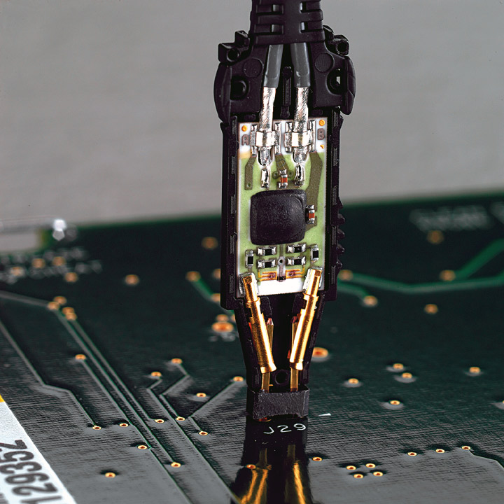
FIGURE A. A general-purpose logic analyzer probe with a 0.025” square wire-wrap type of pin adapter.
High-density, multi-channel probes require dedicated connectors on the circuit board (see Figure B).

FIGURE B. A high-density multi-channel logic analyzer probe.
The probe shown in Figure C can acquire high-quality signals and have a minimal impact on the SUT by clamping on to existing device packages. This type of probe is recommended for applications that require higher signal density and reliable connections to your SUT.
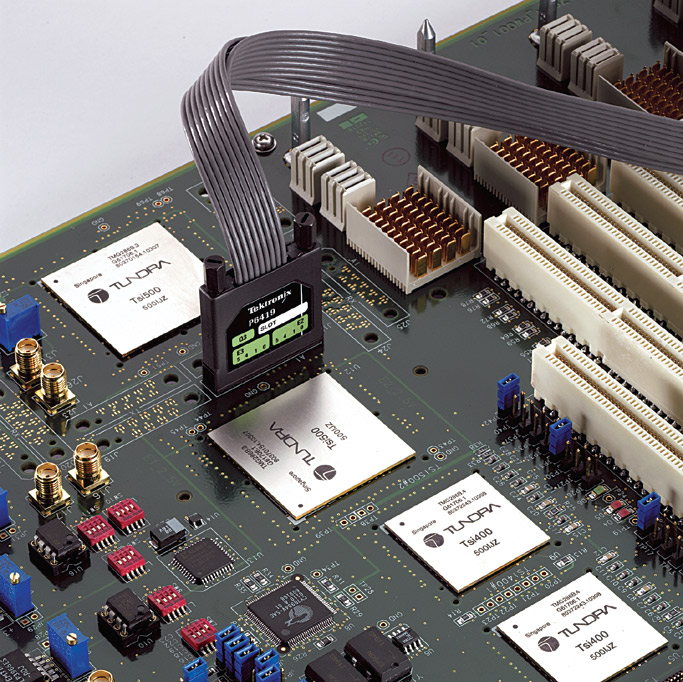
FIGURE C. A compression logic analyzer probe.
Probe impedance (capacitance, resistance, and inductance) becomes part of the overall load on the SUT. All probes exhibit loading characteristics. The logic analyzer probe should introduce minimal loading on the SUT, and provide an accurate signal to the logic analyzer.
Probe capacitance tends to “roll off” the edges of signal transitions (see Figure 5).
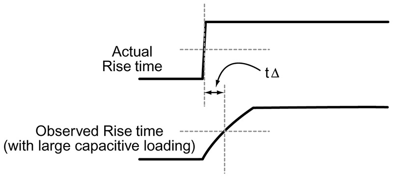
FIGURE 5. An illustration of how the impedance of the logic analyzer’s probe can affect a signal’s rise times and measured timing relationships.
This roll-off slows down the edge transition by an amount of time represented as “t” in the figure. Remember, slower edges cross the logic threshold of the circuit later, introducing timing errors in the SUT. This problem becomes more severe as clock rates increase.
In high speed systems, excessive probe capacitance can potentially prevent the SUT from working. It is always critical to choose a probe with the lowest possible total capacitance. It’s also important to note that probe clips and lead sets increase capacitive loading on the SUT. Use a properly compensated adapter whenever possible. The impedance of the logic analyzer’s probe affects signal rise times and timing relationships.
Logic analyzers capture data from multi-pin devices and buses. The term “capture rate” refers to how often the logic analyzer samples the inputs. It is the same function as the time base in an oscilloscope. Logic analyzer literature interchangeably uses the terms “sample,” “acquire,” and “capture.”
Timing acquisition captures signal timing information. In this mode, an internal clock samples data. The faster it samples data, the higher the resolution of the resulting measurement. There is no fixed timing relationship between the target device and the data the logic analyzer acquires. Use this acquisition mode when you are concerned with the timing relationship between SUT signals.
The acquisition mode acquires the “state” of the SUT. A signal from the SUT defines the sample point (when and how often data is required). The clock signal you use in the acquisition mode may be:
- The system clock
- A control signal on the bus
- A signal that causes the SUT to change states
You sample data on the active edge, which represents the SUT when the logic signals are stable. The logic analyzer samples only when the selected signals are valid. What transpires between clock events is irrelevant.
More on Data Acquisition Modes
There are two types of data acquisition modes: synchronous and asynchronous. For long, continuous records of timing details, use the timing acquisition mode and the internal (or asynchronous) clock. Acquiring data exactly as the SUT sees it requires you to use the state (synchronous) acquisition mode.
In the state acquisition mode, the logic analyzer displays each successive state of the SUT sequentially in a window. You may use any relevant signal for the external clock signal for state acquisition.
Triggering selects which data you capture. Logic analyzer triggering only occurs on digital signals, and is more sophisticated than triggering on any oscilloscope.
Logic analyzers can recognize Boolean operators, such as multiple signals that are “AND”ed or exclusive-”OR”ed together, etc. They can track SUT logic states and trigger on conditions within the SUT that you desire. These may be a simple transition — intentional or otherwise — on a single signal line.
If you are chasing an elusive glitch that occurs when an Increment or Enable pin becomes valid, you might want to trigger on some set of bus-wide conditions that are known to preceed it. This is a powerful feature of a logic analyzer.
In all instances, the “event” appears when signals change from one cycle to the next. You can use many conditions to trigger your logic analyzer, such as a specific binary value on a bus or counter output. Other triggering choices include:
- Words: Specific logic patterns defined in binary, hexadecimal, etc.
- Ranges: Events that occur between a low and high value.
- Counter: The number of events you program that you are tracking by a counter.
- Signal: An external signal such as a system reset.
- Glitches: Pulses that occur between acquisitions.
- Timer: The elapsed time between two events or the duration of a single event, tracked by a timer.
- Analog: Use an oscilloscope to trigger on an analog characteristic and to cross-trigger the logic analyzer.
With all these trigger conditions available, it is possible to track down system errors using a broad search for state failures, before you refine your search with increasingly explicit triggering conditions.
I hope this introduction has taught you a few things about this powerful benchtop tool — look forward to more in Part 2! NV