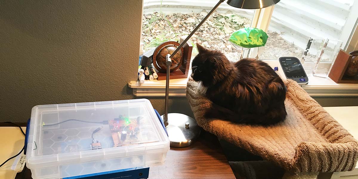
My cat, Maxwell (top graphic; Figure 1), has an overactive thyroid; a condition called hyperthyroidism. The cure for him has been giving him pills of Methimazole. All cat owners know that giving a cat a pill is no fun for anybody. When he requires four pills a day and each one costs $0.50, it’s like shoving two dollar bills down his throat every day. It’s even more expensive when the pills are ground up in tuna.
A web search revealed there is another treatment for hyperthyroidism with a 95% success rate in cats, based on radioactive Iodine-131. The idea is to kill off the overactive regions of the thyroid with radiation. Because the thyroid selectively absorbs iodine, a radioactive form of iodine is injected into the cat. It concentrates in the thyroid and over a few weeks, kills off some of the thyroid. When done correctly, this is a permanent cure. However, it means making him radioactive, but only for a few weeks.
Radioactivity and Iodine
Every element on the periodic table has just one unique atomic number. This is the number of protons in its nucleus; the same as the number of electrons in the atom. The atomic number of iodine is 53. Iodine can have a wide range of neutrons in its nucleus. We call these different forms of iodine (with different numbers of neutrons) isotopes.
There are 37 known isotopes of iodine — all with 53 protons in the nucleus, but with 55 to 93 neutrons. We track the total number of particles in the nucleus as the atomic weight. For iodine, it varies from I-108 to I-144.
All these isotopes are radioactive except I-127, which is stable. Iodine-131 has special use in medical treatments. This is partly because iodine is biologically active and is selectively taken up by the thyroid. It is a beta and gamma emitter with a half-life of eight days. This is perfect for targeted radiation attacks on thyroid cells.
There are three types of radioactive particles emitted in radioactive decay: alpha particles, which are two protons and two neutrons; beta particles, which are high energy electrons; and gamma particles, which are high energy light photons.
Alpha particles have the potential to produce the most biological damage, but they don’t penetrate much more than the thickness of a piece of paper. However, if the radioactive source is ingested or inhaled, it can do a lot of local cell damage.
Radon is a noble gas which decays and emits alpha particles. Breathe it in and it decays in your lungs, and you have a higher chance of contracting lung cancer. This is why we test for radon in basements where it's a decay product of uranium into radium, and then into radon, naturally occurring in bedrock.
Beta particles don’t penetrate more than a quarter of an inch in tissue. This means that if they can be placed strategically in tissue you want to kill off, they will deposit all their lethal effects very localized. Beta emitters make the perfect surgical strike killers.
Gamma particles are just a form of light but of very short wavelength, or high energy per photon. They travel much farther through the body and through air than beta particles. These will make it out through the body and are used to image deep tissue. This is the basis of PET (Positron Emission Tomography), for example.
You’re injected with a biologically active material that emits positrons — an anti-electron. As soon as it is emitted, it immediately annihilates with the first electron it encounters, and the pair gives off two gamma particles which make their way out of the body and are detected.
Iodine-131 decays into Xenon-131 by emitting a beta particle with energies ranging from about 190 keV to 606 keV. This is what does all the medical work. This is a lot of energy to be deposited locally into the targeted tissue.
The new Xenon nucleus is created in an excited nuclear state. Immediately after the neutron emits the beta particle and decays into a proton, the new proton jiggles around, drops down to a ground state, and emits a gamma particle with an energy of 364 keV.
By comparison, a dental x-ray may be as high as 70 keV. This 364 keV gamma ray particle makes its way outside the body and we see it as “radiation.” With I-131, we get a 2-for-1. The beta particle does the therapeutic work and the gamma particle allows us to see it in action. Every gamma particle we detect means there was a beta particle killing off thyroid tissue.
The half-life of I-131 is eight days. This means every eight days, the number of I-131 atoms left is reduced in half, and the rate of decay has decreased by half. After 16 days, there are about 1/2 x 1/2 or 25% of the starting number of I-131 atoms left, which means the radiation emitted is reduced to 25%. After 60 days (or about eight half-lives), there is only 1/ 2^8 = 0.4% of the radiation levels as initially.
I expected Maxwell’s radiation levels to drop off faster than an eight day half-life because he was constantly losing radioactive iodine from his body as it cycled through. It was flushed out of his system and ended up in his kitty litter, which would also be radioactive.
The vets at the clinic warned us not to spend much contact time with Maxwell until his radiation levels dropped and to not throw his litter out in the trash. They said the radiation levels in his used cat litter might set off radiation detectors at municipal dumps.
I wanted to build a radiation detector to see how hot Maxwell was initially, and how quickly his radiation levels (and his used cat litter) dropped off.
Detecting Radiation
Since I was only going to detect gamma particles, a Geiger counter was the obvious detector choice. The original name for the detector is really a Geiger Muller tube, named after Hans Geiger and Walther Muller, who developed the detector in 1928. It’s sometimes referred to as a GM tube, including both inventors.
A GM tube is basically a vacuum tube with about 1/10 an atmosphere of air. A central wire (the anode) is at a high positive voltage, while the outer metallic cylinder (the cathode) is at a lower voltage. When a particle like a gamma particle or beta particle passes through the thin gas, it leaves a trail of ions and electrons behind it. The ions accelerate to the lower voltage outer shell (the cathode).
If the voltage is high enough and the gas pressure is just right, the ions collide with more air molecules and ionize them; they get accelerated and ionize more; and we get an avalanche and a large current burst. This avalanche multiplies the original number of ions created by the gamma particles by a factor of 100 or more. It self-terminates in a micro second or so.
There are Geiger tubes for sale from scientific supply houses, but they range in price from $100 to more than $300. However, when you do a web search for Geiger tubes, the first items that come up are vintage Soviet military Geiger tubes on eBay for only $5-$20. These were used by Soviet soldiers when investigating potentially hot areas.
I went ahead and purchased two of the STS-5 Geiger counter tubes (shown in Figure 2) which had never been used. I paid $16 for each one.
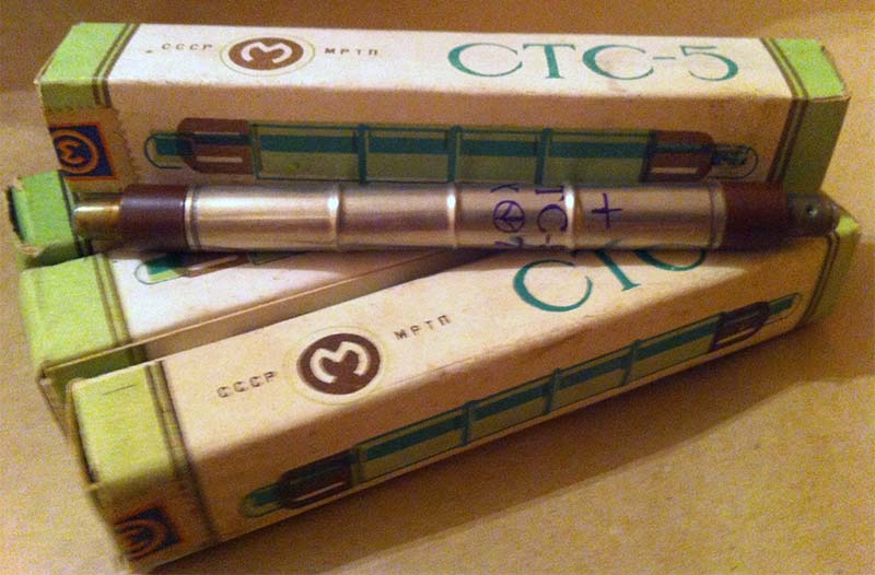
Figure 2. Soviet military surplus Geiger tubes and their packaging.
The specs say the Geiger tube operates between 280V to 390V. The background rate is about 25 counts per minute, with a max count rate of about 150,000/min.
These units are shipped from the Ukraine. When the package arrived with the Ukraine return address and Cyrillic writing, my wife warned me that we were probably on a Homeland Security list somewhere. When I mentioned I might be ordering some radioactive samples to test my Geiger counter, she drew the line and told me she did not want a “visit” from Homeland Security. I had to make do with something else.
The next step was to build the electronics to power-up the Geiger counter and count current pulses, record the counts, and convert to counts per minute to be plotted directly into Excel.
The High Voltage Circuit
Since I am enamored with the power of the Arduino, my detector was going to be Arduino based. I didn’t need anything very sophisticated so decided on an Uno, which is my workhorse general-purpose Arduino. I use this microcontroller in the workshops I teach at our local hackerspace, Tinkermill. In my three years of teaching this workshop — with more than 300 participants and all of my playing around, plus Maxwell as my ESD tester — I have never damaged an Uno. Until this project.
I blew two Arduinos by accidently touching a digital pin to the 50V on the low side of the high voltage supply. I was very careful after this.
The Geiger tube takes about 300V. This voltage level with its capacitance can be lethal! DO NOT ATTEMPT THIS CIRCUIT UNLESS YOU ARE EXTREMELY CAREFUL!
As a special precaution, I built the entire circuit inside a plastic box (Figure 3) which I could seal up, and keep fingers and cat noses and tails from touching anything that might be high voltage.
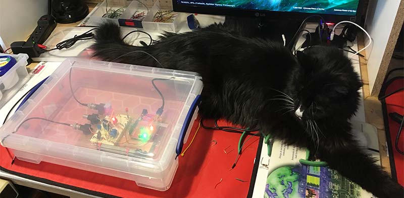
Figure 3. The Geiger counter circuit and tube are inside a sealed plastic box for safety and convenience. Note the battery connection for portable operation.
This also made the project transportable and easily handled.
This circuit has three parts: the high voltage generator; the detector circuit; and the pulse output circuit. I wrote the sketch to control the high voltage, count the pulses, and print the counts per minute directly into Excel.
I wanted to generate a stable voltage across the anode and cathode with low noise and an adjustable value from about 250V to 400V. When I looked at high voltage generator circuits for Geiger counters on the Web, they were almost all based on a boost circuit and transformer using a 555 timer with a fixed frequency. This would be okay if I just wanted a fixed voltage, but I didn’t know what voltage would work best with these Soviet Geiger tubes.
So, I decided to design my own boost circuit, but take advantage of the audio transformers used in most of these. I used to be able to get these small form factor 10:1 transformers from RadioShack (Figure 4).
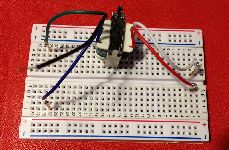
Figure 4. RadioShack audio output transformer.
I bought the last three units. I figured I was going to use an Arduino anyway, so why not use it to control the pulses through the boost circuit based on the voltage on the supply. It would act as a “smart” digital power regulator.
The circuit is shown in Figure 5.
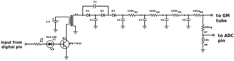
Figure 5. Circuit for the high voltage power supply.
The principle is simple: A short 5V digital pulse from an Arduino pin turns the transistor on briefly. This sends current through the inductor. The voltage across the inductor is clamped by the 5V supply on one side and on its other side, the low impedance of the on-transistor tied to ground.
When the transistor turns off, the current through the inductor suddenly stops and the back EMF voltage generated across the inductance of the primary winding goes very high, limited by the maximum collector-emitter breakdown voltage of the transistor. This is about 50V for the transistor I am using.
This means I get a 50V voltage pulse on the primary winding, or a 500V pulse on the secondary windings. The turns ratio for this simple audio transformer is 10:1. This 500V pulse on the high side is rectified by the initial diodes and then gets dumped into a 10 nF capacitor. The capacitor smooths out the pulses into a more steady value. Since I am using potentially 500V, I made sure my diodes and capacitors had a 1 kV rating.
This is basically a peak detector circuit with a little voltage boost. I added a 10 meg load resistance so there would be a constant bleed off of voltage from the last capacitor. The time constant of the 4 x 10 nF capacitor and 10 meg resistor is 0.4 sec. This means once pulses stop entering the transistor, the voltage across the GM tube would drop to nearly zero in about two seconds. This is a good safety feature!
Each pulse dumps a little charge into the capacitors. If the transformer pulses dump charge into the capacitors faster than the 10 meg resistor drains it off, the voltage increases. I had to send pulses often enough to charge up the capacitor. I read the voltage across the capacitor with an analog channel. I only send pulse trains out to the transistor when the voltage on the capacitor is below the set-point voltage.
Of course, I couldn’t connect the ADC (analog-to-digital converter) input pin directly to 500V. I’m limited to a max of 5V on the ADC pin. I used a 1,000:1 attenuator using the 10 meg bleed resistor and a 10K resistor in series.
The voltage across the 10K resistor is 0.001 x Vcap. A 100V rail is recorded as 0.1V on the ADC pin. With 10-bit resolution on the ADC, I have a resolution of 5 mV on the ADC. This translates to 5V resolution on the voltage rail. This is plenty good.
I added one other feature. I wanted a clean stable voltage on the Geiger tube. With all these pulses, I was getting too many spikes. I added a three-stage RC filter on the output of the rail. Each capacitor is 10 nF, and I wanted a 1 ms time constant, so I used 100K resistors in each stage.
By experimenting around, I found that a pulse width driving the transistor of about 0.5 ms was the minimum width to get the full voltage across the inductor. The fastest they would be generated is 1 kHz.
For these sorts of pulses, a scope is an essential lab instrument tool. One of my favorite lower end scopes is the Picoscope 2204A: an eight-bit 100 Msample/sec scope with a list price of $129 shipped with their standard scope software. Figure 6 shows the voltage on the rail with the 1,000x attenuator and the pulses to the transistor, while the voltage is being regulated at 310V.
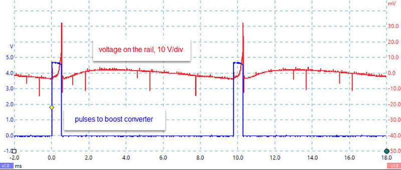
Figure 6. Voltage pulses into the transistor and the output voltage rail with just background counts.
Each pulse increased the voltage on the rail; while between pulses, the voltage drooped due to the 10 meg bleed resistor.
I like feedback. I added an LED in series with the digital signal to the transistor that triggers the high voltage. This way, I can glance at the board and confirm by the lit LED that pulses are going to the high voltage generator.
Pulse Detection Circuit
Each ionization avalanche causes a brief current pulse through the Geiger tube to ground. To measure this current pulse, I passed the current through a 10K resistor and measured the voltage pulses on my scope. A 1V pulse means 0.1 mA of current. Figure 7 shows a few of these pulses. The scope limit is 20V on this scale.
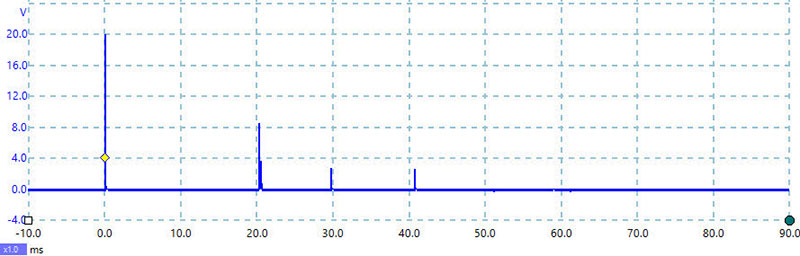
Figure 7. Current pulses from the Geiger tube with a source nearby showing current peaks from 0.4 mA to 2 mA.
The pulses are typically greater than 0.5V across the 10K resistor. Just to give a little bit of margin, I used a 100K resistor across the transistor base in the detector circuit. The exact value wasn’t important, as long as the voltage pulses were above 0.6V — enough to turn on the transistor and pull the Arduino pin down.
I set up the Arduino digital pin as an input using the INPUT_PULLUP mode. This ties the input receiver on the pin to the +5V line through a 10K resistor. Normally, when the transistor is off, the input voltage read is a logic 1 at 5V. When the transistor turns on from a detected current pulse, the input to the pin is pulled low and seen as a low by the Arduino.
I used an interrupt function to react to the falling edge signal picked up on one of the digital input pins. When a falling edge is detected, the function in the interrupt increments a counter and waits for 8 ms as a dead time. In the avalanche process, sometimes double pulses are created due to secondary breakdown in the gas. Adding this 8 ms delay avoids any double counting. It also increased the dead time.
For example, if in 60 seconds, there are 600 counts, the count rate is 600 counts per minute. The dead time is 600 x 10 ms = 6 sec, or 10%. For lower count rates, the dead line is less. For higher count rates above 600 counts/min, the dead time will increase and we may not get an accurate count rate.
Each time I detect a pulse, I also flash an LED pulse and I click a buzzer. After all, what’s a Geiger counter without a clicking sound?
Exporting to Excel
I love numbers. If math is the language of theoretical science, measurements are the language of experimental science. Measurements are especially valuable when we can bring them into Excel and analyze them. In searching on the Web, I came across an invaluable free tool which allows me to write data directly into an Excel spreadsheet. I’ve written about this in Nuts & Volts a few times (see Resources).
The application is called PLX-DAQ v2 and is basically an Excel file with a macro that reads the serial port and parses the printed values into cells (see Resources for a link to download an Excel file with this macro embedded).
I wrote a sketch to count pulses in 10 sec intervals, then calculate the counts per minute and print these values every 10 seconds to Excel. In Excel, I plot the count rate over time. Figure 8 is an example of the count rate measured over a period of six hours while monitoring Maxwell in his cat tree apartment.

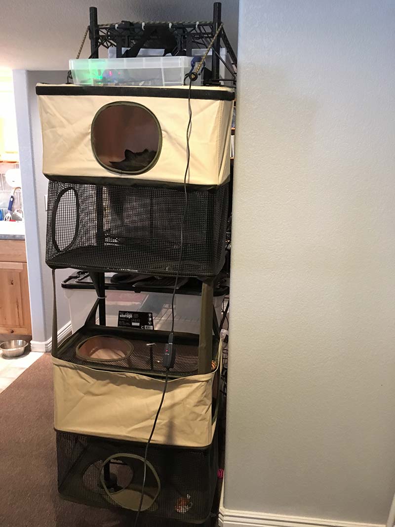
Figure 8. Count rate measured while Maxwell was in his cat apartment. He can be seen inside the top hole. The Geiger counter is right above him.
My Prototyping Philosophy
From my years of experience in startups and product development programs, I’ve embraced the motto, “Fail often and fail early.” This means I want to design and build a prototype with the best practices I can think of, but get it done quickly. Then, I can use the prototype to test my approach. I want to use my prototype to help me find the things I could not anticipate, so the next versions get better and better.
When I build Arduino circuits, I always start out building them on a solderless breadboard. It takes minutes to put something together and test out. Figure 9 is the prototype Geiger counter that I put together in about three hours.
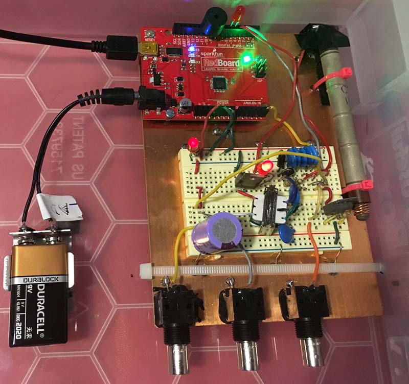
Figure 9. Example of building a relatively complex circuit using a solderless breadboard. The entire circuit took about three hours to design, build, debug, and optimize.
It is so much quicker than designing a circuit board, sending it out to get made, and assembling it. When I have a final stable design and may want to make multiple units, I will design a board at that time.
The downside to using a solderless breadboard is that it may have more noise and not as good signal integrity as a multi-layer circuit board. This is one reason I mount my solderless breadboards on a copper base connected to ground. I keep wires short and route signal lines close to the copper base, and pay attention to all signal return paths. In other projects, I’ve been able to keep voltage noise levels from AC and RF pickup below 1 uV RMS.
My designs may not look pretty, but I can construct them quickly, make changes on-the-fly, and optimize the design in hours instead of weeks. They have surprisingly good performance.
Testing My Geiger Counter
When I turned on the voltage to my Geiger counter, I immediately began detecting pulses when the applied voltage was above 290V. I settled on 310V as giving a steady rate of pulses, at about 30-50 counts per minute. This was the background I expected to see, but was it really detecting radiation?
I needed a radiation source to test my Geiger counter (remember my wife forbade me from ordering anything that could potentially trigger a Homeland Security alert). Turns out, I could buy one at Walmart.
There are two types of smoke alarms: photoelectric based and ionization based. The ionization based smoke detectors have a small piece of Americium-241. It is radioactive, and emits an alpha particle and a very low energy gamma particle. The gamma particle has an energy of 59 keV which is in the range of dental x-rays. I had no hope of detecting the alpha particle, as it would be stopped by the metal wall of the Geiger tube. However, I thought I might be able to detect the low energy gamma.
I bought an ionizing smoke detector for $7 and took it apart. I found a piece of metal that looked like it could be the ionizing source. I pulled this off the detector and brought it close to the Geiger counter (shown in Figure 10).
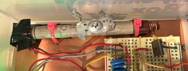
Figure 10. Americium source pulled from a smoke detector and placed on top of the Geiger tube.
To my delight, the buzzer starting buzzing and the LED light started flashing. When the source was right on top of the Geiger tube, the count rate was 950 counts per minute, as compared to about 45 counts/min as background. My detector was working! A recording of this source is shown in Figure 11.
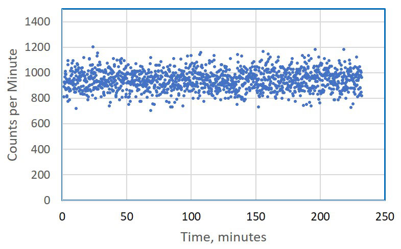
Figure 11. Background count rate and when the smoke detector source is on top of the GM tube.
Maxwell is Hot
One week after his injection of I-131, we picked up Maxwell at the vet and brought him home. It was a little hard to get him to stay still long enough to measure his count rate. I had cut the counting interval down to 10 seconds, but I still needed the cat to stay still for a few minutes to get good statistics. Figure 12 shows my first attempt to get a reading on Maxwell.
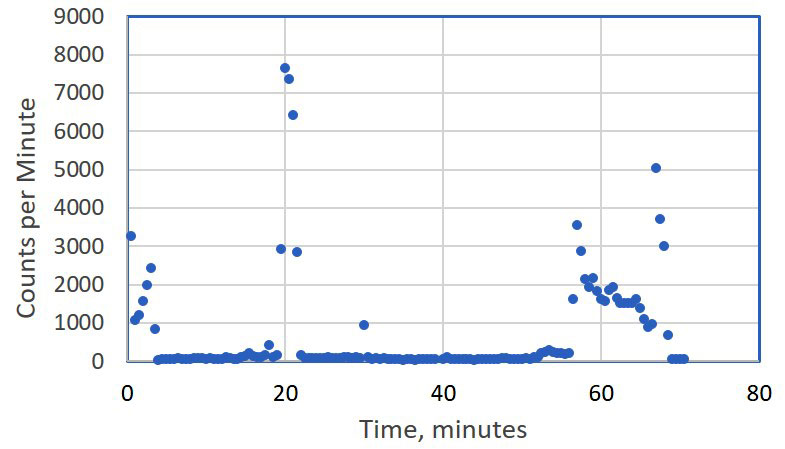
Figure 12. First reading of counts from Maxwell. He was at more than 6,000 counts per minute -- almost at the measurement limit!
I found early on that his count rate was strongly dependent on how close he was to the detector. To get stable and reproducible readings and compare his count rate changes each day, I decided on measuring him with a fixed distance of 12 inches from his neck. I also waited for him to settle down in one of his favorite napping locations. Figure 13 shows the typical setup I used to get reproducible measurements.
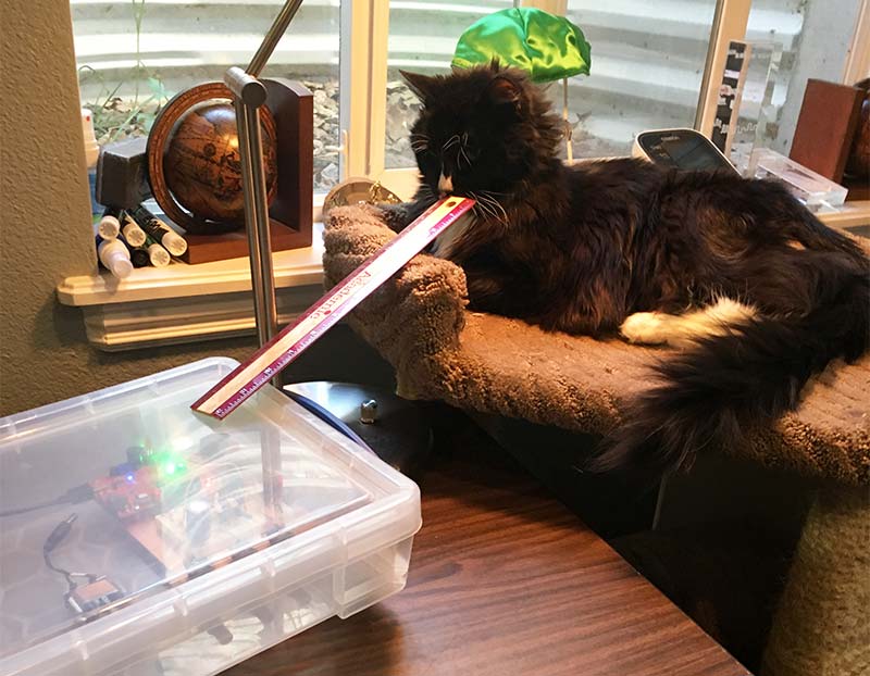
Figure 13. Maxwell napping while I measured his count rate with the detector 12 inches from his neck.
On his fourth day home, his count rate was about 850 counts per minute at 12 inches. Figure 14 shows these initial stable readings.
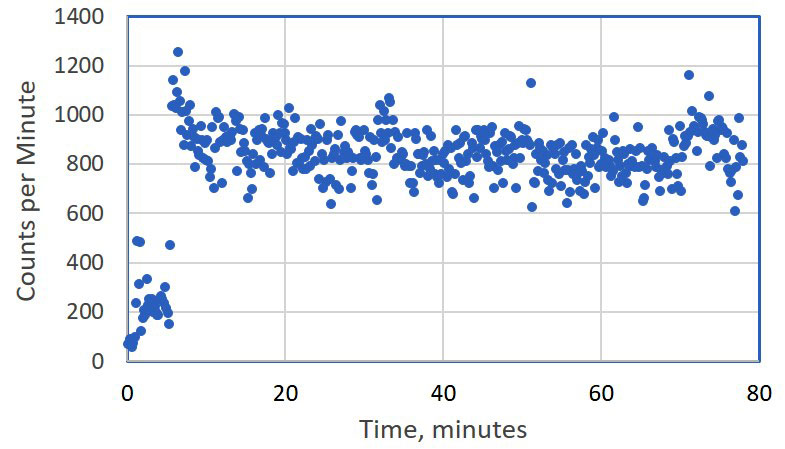
Figure 14. Maxwell at 12 inches, with about 850 counts per minute average reading on day four.
On day 11, Maxwell was down to 160 counts per minute. By day 13, he was down to 92 counts per minute — only twice above background. Unfortunately, his poop wasn’t.
What Do You Do with Radioactive Kitty Litter?
Part of the reason Maxwell’s counts dropped so fast was that he was excreting a lot of the radioactive iodine. This meant his kitty litter was radioactive. I scooped up the first sample and kept it in a bag to use as a reference. The decay rate of this clump should reflect the decay rate of I-131. I kept this around my lab and measured it periodically, trying to be careful to keep it the same distance from the detector each time.
I used the lid of the plastic box of the Geiger counter as the reference position. Figure 15 shows the sample resting in the detector box while I took readings for an hour to get good statistics.
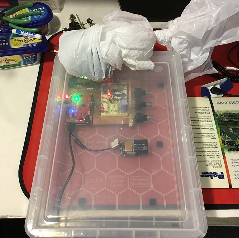
Figure 15. Measuring the first kitty litter sample with a precision distance from the detector.
With a count rate of about 600 counts/min over one hour, I collected about 36,000 total counts. The standard deviation on this is about sqrt(36,000) = 190 counts/per hour = 3 counts/min. My statistical noise on the decay rate for this sample was about 3 counts/min, or a little less than 0.5%.
In the first sample as a reference, I can measure the half-life of I-131. Every few days, I measured the count rate of this sample over a one hour period. This gave good statistics. I then plotted up the count rate in counts per minute, averaged over at least one hour. This is plotted on a semi-log plot in Figure 16.
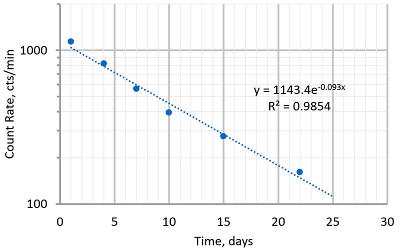
Figure 16. Decay rate of the first kitty litter sample averaged over one hour, measured for three weeks.
When plotted on a semi-log plot, the exponential decay rate is a straight line. I fitted an exponential decay rate and got a decay rate of 10.75 days.
The half-life is calculated as the exponential decay rate x ln(2) = 7.45 days. This is pretty close to the 8.03 day reported half-life of I-131. I might have gotten a more accurate value if I was more careful in preparing the sample instead of just casually throwing it on top of the lid. The position of the sample and the distance to the detector is an important factor influencing the measured count rate.
In addition, I did not do a very good job of tracking the exact time of day I performed the measurement. The precise time of each measurement could be off by as much as 0.25 days.
After the first few days, I’d collected enough used kitty litter to bag up. Sure enough, it was hot. I was getting counts of more than 500 counts/min with the detector close to the bag. I had a five gallon pail with a sturdy lid in the back yard to store the used kitty litter until the count rate dropped down. I estimate this will be in about four half-lives, or about one month. The count rate will be just above the background by then and I can send it to the municipal dump.
Prognosis
Maxwell came through his procedure with no complications. One month after his treatment, his thyroid and blood work had him almost back to normal. The vet says we have to wait six months after the procedure for the final verdict.
In the meantime, I have some other experiments planned with my Soviet military surplus Geiger counter. Assuming Homeland Security doesn’t come knocking. NV
Resources
“Why You Need an Analog Front End and How to Set It Up,” Eric Bogatin, Nuts & Volts.
“Turn Your Microcontroller into a Precision Data Acquisition System,” Eric Bogatin, Nuts & Volts, June 2017.
“Special Day for Physicists Cats,” Eric Bogatin, EDN news portal, August 12, 2013 (www.edn.com/electronics-blogs/test-voices/4419602/Happy-birthday-Schrodinger).
Iodine 131 treatment: https://vcahospitals.com/alameda-east/specialty/search-results?term=Iodine%20131%20treatment.
RadioShack audio transformer: https://www.ebay.com/p/132000355.
Picotech P2204A scope: https://www.picotech.com/oscilloscope/2000/picoscope-2000-specifications.
"Arduino Based Data Acquisition," Eric Bogatin, Nuts & Volts.
Link to download PLX-DAQ v2: http://forum.arduino.cc/index.php?topic=437398.msg3172623#msg3172623.
Parts List
| QTY |
ITEM |
| 1 |
Arduino Uno |
| 1 |
Solderless breadboard |
| 1 |
RadioShack 273-1380 audio output transformer |
| 1 |
TIP31 NPN transistor |
| 2 |
Red LEDs |
| 3 |
1N4007 1 kV diodes |
| 5 |
10 nF 1 kV ceramic capacitors |
| 5 |
100K resistors |
| 1 |
10 meg resistor |
| 1 |
1 meg resistor |
| 1 |
10K resistor |
| 1 |
1K resistor |
| 1 |
Arduino piezoelectric buzzer |
Downloads
What’s in the zip?
Source Code