The popularity of repairing and restoring tube radios has highlighted the need for a variety of test instruments. A voltmeter and signal generator are essential for troubleshooting. A wide-band oscilloscope comes in handy at times for tracing signals in radio frequency (RF) and audio circuits.
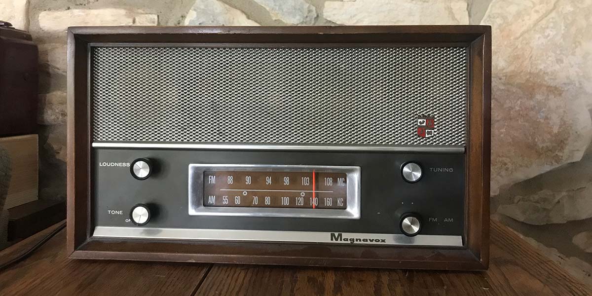
After repair or restoration of a radio, the final step is often alignment. For an AM radio, a signal generator and voltmeter will do a good job. But with an FM radio, using a signal generator and voltmeter does not always produce the best results. This came home to me some time ago after restoring a very nice Magnavox AM/FM tabletop radio shown in Figure 1.
FIGURE 1. Classic Magnavox AM/FM radio (model FM-21).
Following the Sam’s Photofact AM alignment procedure using a signal generator/voltmeter, AM alignment went without a hitch and the radio’s performance was excellent. FM alignment was not as successful. The Sam’s Photofact service documentation gave two FM alignment procedures: one using a signal generator and voltmeter; the other using a sweep generator and oscilloscope. Not owning a sweep generator, I used the signal generator/voltmeter procedure.
When finished, I tuned in a local FM station. To get the clearest audio, I had to tune slightly off the station’s frequency. Even then, the audio was not up to FM quality standards.
I suspected the problem was alignment but without a sweep generator, I was stymied. Thinking I might find a bargain sweep generator, I checked online for sellers. Nothing in my budget range came to light. I began tossing around ideas about the possibility of building an all-in-one sweep alignment instrument using a digital signal generator module, Arduino processor, and digital display. The crucial question was whether a digital signal generator module could change frequency rapidly enough to provide a real time display of the sweep response.
A little research revealed that the readily available AD9850 DDS (Direct Digital Synthesis) module would work. Not only could the output frequency be changed quickly enough, but the DDS module was readily available and reasonably priced at $25. With this information in hand, I launched my project to design and build a self-contained sweep alignment instrument. I christened it the WhippleWay Sweep Alignment Board or WSAB, for short.
During the succeeding year, the WSAB passed through several revisions, finally reaching a satisfactory level of performance late in 2020. In the new year, I collected the knowledge gained and published the Amazon book, Vintage Radio Alignment — From Scratch. This article is a “digest” of that book. If you want a more in-depth treatment of radio alignment, I recommend the book.
To cover sweep theory and practice plus construction of the WSAB alignment instrument, I must present the article in two parts. In this issue, I’ll cover sweep theory and construction/operation of the WSAB. In the next issue, I’ll cover sweep alignment procedures for both AM and FM, plus an example of each.
Basic Alignment Theory
Before describing my sweep instrument project, a brief look at the theory of vintage radio alignment is in order. Figure 2 shows a block diagram of a typical superheterodyne radio, either AM or FM.
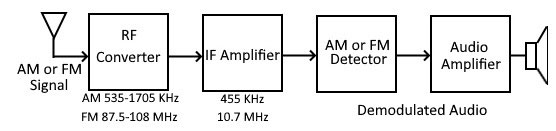
FIGURE 2. Superheterodyne receiver block diagram.
The received station’s RF signal is converted to an intermediate frequency (IF) signal, amplified, detected, then passed as demodulated audio to an audio amplifier and the speaker. RF and IF stages contain filter circuitry that selects a single station’s signal for reception, isolating it from adjacent station signals. A radio’s capability to do this is known as “selectivity.”
While some selectivity is provided by a tuned circuit in the RF converter, it’s primarily achieved by multiple tuned circuits in the IF amplifier. Because of the variability in off-the-shelf components during manufacture, radio designs include a way to adjust the RF and IF tuned circuits for optimum performance. The procedure for making these adjustments is referred to as “alignment.” Alignment of the RF converter is called “tracking alignment;” that of the IF amplifier is called “IF alignment.”
As the vintage radio ages, components drift in value and realignment is often necessary. This is particularly true of FM radios because of the higher RF and IF frequencies they must handle.Selectivity requirements and alignment procedures for AM and FM differ, so they will be discussed separately beginning with AM.
AM IF Selectivity and Alignment
The most common IF frequency for AM is 455 kHz (see Sidebar 1).
Sidebar 1
The choice of AM IF frequency is based on two principal factors. First, it must be far enough below the lowest AM band frequency not to cause tuning interference. Second, it can’t be too low as this results in multiple images of the received or other stations falling within the AM 535 to 1705 kHz band.
Over time, several IF frequencies were adopted. Early AM all-triode superhets utilized frequencies as low as 175 kHz to obtain satisfactory gain and stability. Later, with the development of high gain pentodes, 455 kHz became the recognized standard.
The choice of FM IF frequency was first 4.3 MHz when the first FM band was first established in the 40 to 50 MHz band. Later, when the FM band was moved to its current location — 88 to 108 MHz — 10.7 MHz was settled on as the standard IF frequency.
Figure 3 shows the IF response curve for a typical AM radio.
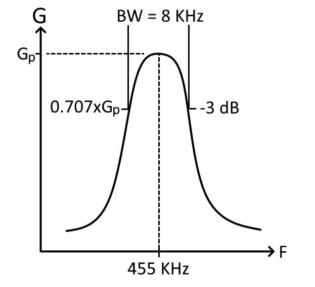
FIGURE 3. IF response curve for an AM radio.
A “response curve” is a plot of IF amplifier voltage gain (vertical axis G) versus frequency (horizontal axis F). Voltage gain is given by dividing the IF output signal amplitude (Aout) by the IF input signal amplitude (Ain).
Because voltage gain can range from fractions up to very large numbers, this formula is applied to compress the range to more convenient values:
Selectivity of a peaking response curve like the one shown is often specified by stating its “bandwidth.” Bandwidth (BW) is defined as the difference between the upper and lower frequencies where power gain is one-half that at the peak. This occurs when the voltage gain is down by a factor of 0.707 or -3 dB. IF filters are designed so that beyond the -3 dB frequencies, gain falls off rapidly and adjacent station signals are greatly attenuated.
For amplitude modulation, the response curve must include the station’s carrier plus two “sideband” signals located at the carrier frequency, minus the audio content frequency and the carrier frequency, plus the audio content frequency. (Refer to Sidebar 2.)
Sidebar 2
An amplitude modulated (AM) signal consists of RF energy at the carrier frequency and at sideband frequencies given by the carrier frequency, minus the frequency of the audio content and the carrier frequency, plus the frequency of the audio content. The carrier is always present while the sidebands come and go with audio content.
The dotted line in Figure A is the ideal IF response curve to receive the turned station based on a maximum audio content frequency of 5 kHz.
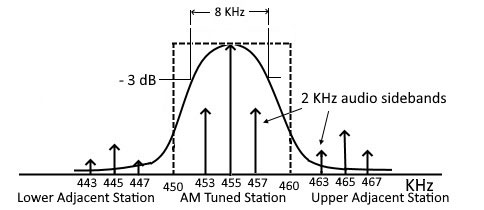
FIGURE A. AM spectrum of station tuned and adjacent stations.
Only the carrier and sidebands of the tuned station are within the passband of the response curve. The solid line is representative of an actual IF response curve. Note that with 10 kHz station separation and audio frequencies less than 5 kHz, station signals don’t overlap, and the actual response curve provides significant attenuation of adjacent station signals.
Most AM stations consider the audio content maximum frequency to be 5 kHz requiring a 10 kHz bandwidth to capture the resulting sidebands. While this gives good fidelity for speech reproduction, it’s somewhat limiting for music reproduction.
A bandwidth of 8 kHz is a reasonable compromise between fidelity and selectivity. While audio above 4 kHz falls off somewhat — more importantly — adjacent channel attenuation reaches an acceptable level. To compensate for this, some AM stations boost audio frequencies above 4 kHz, not that this achieves much. The fact is that most vintage radios don’t have the audio capability to reproduce audio in this higher range anyway.
Historically, AM IF frequencies have varied from 100 kHz to mid-400 kHz. The lower IF frequencies were around when triode tubes prevailed, and much attention was given to their lack of gain and instability at higher frequencies. With the introduction of high gain and stable pentode tubes, 455 kHz was eventually settled on as the standard. At 455 kHz with an 8 kHz bandwidth, only a single IF stage consisting of a tube and two double-tuned IF transformers is needed. The tube provides needed gain, while four tuned circuits (two within each IF transformer) provide a response curve that meets the bandwidth requirement.
AM IF alignment involves adjusting the IF tuned circuits to resonate at 455 kHz. By design, doing so produces the correct response curve. Two non-visual alignment methods are commonly employed. The first method uses a signal generator and an AC/DC voltmeter or an oscilloscope. A modulated 455 kHz signal is injected before the first IF transformer and demodulated audio is monitored at the speaker using the AC function of the voltmeter or the oscilloscope. The IF transformers are tuned to peak (maximize) the level of demodulated audio.
The second method relies on the fact the AM detector produces a DC output voltage proportional to the amplitude of the injected 455 kHz signal. This automatic volume control (AVC) voltage is used to control RF and IF gain and prevent overloading. For this method, an unmodulated 455 kHz signal is injected before the first IF transformer and the AVC voltage is monitored using the DC function of the voltmeter. The IF transformers are tuned to peak the AVC voltage.
In both cases, it’s important to keep the injected signal level as low as possible to avoid overloading and detuning the IF stage. Too high a signal distorts the response curve shape leading to misidentification of the true peak.
FM Alignment
The limited fidelity of AM was in part the impetus for the creation of FM broadcasting. Frequency modulation afforded three distinct advantages: (1) much improved fidelity with an audio frequency range of 20 to 20,000 Hz; (2) high immunity to amplitude induced noise; and (3) low harmonic distortion, typically less than 1%. FM’s higher carrier frequency range (88-108 MHz) requires a higher IF frequency. (See Sidebar 1 again.) The standard in the US is 10.7 MHz. For FM, the instantaneous transmitted frequency varies in accordance with the frequency of the modulating audio. At the same time, the amount of frequency deviation follows the loudness of the audio.
By Federal Communication Commission (FCC) standards, US FM stations must limit maximum frequency deviation to 75 kHz on either side of the carrier. This suggests a minimum bandwidth of 150 kHz. To accommodate FM sidebands, however, more bandwidth is needed. For high fidelity reproduction, a full 190 kHz is needed. (Refer to Sidebar 3.)
Sidebar 3
An FM modulated signal has an infinite number of sidebands diminishing in amplitude as they extend in both directions from the carrier frequency. Obviously, a fixed bandwidth IF response curve will eliminate some sidebands. Most FM signal power (about 98%), however, lies within the bandwidth approximated by Carson’s Rule: BW=2(fd+fm) where fd is the maximum deviation frequency and fm is the maximum modulating audio frequency.
For fd = 150 MHz (the FCC limitation) and a maximum audio frequency of 20 kHz, the Carson bandwidth is 190 kHz. The dotted line in Figure B is an ideal response curve for FM having a bandwidth of 200 kHz.
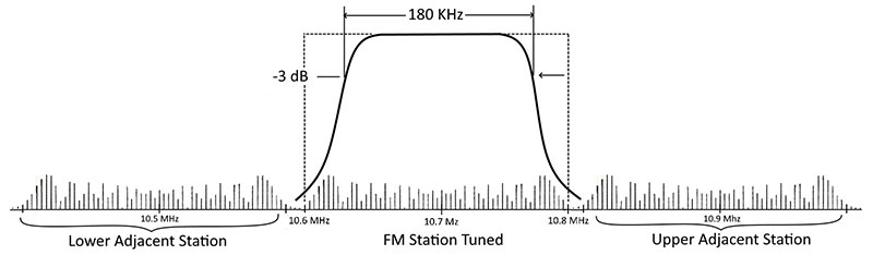
FIGURE B. FM spectrum of station tuned and adjacent stations.
It passes the carrier and Carson sidebands and rejects those of adjacent stations.
The 200 kHz bandwidth is the basis for the FCC’s 200 kHz station allocation standard. The solid line is an FM response curve with a 180 kHz bandwidth. The wide flat response curve coupled with steep sides provides good fidelity along with significant adjacent station rejection.
Also, the FCC allocates FM stations 200 kHz apart allowing 100 kHz either side of the carrier frequency. The FM response curve of Figure 4 with a bandwidth of 180 kHz strikes a good compromise between the 190 kHz bandwidth requirement and adjacent station attenuation.
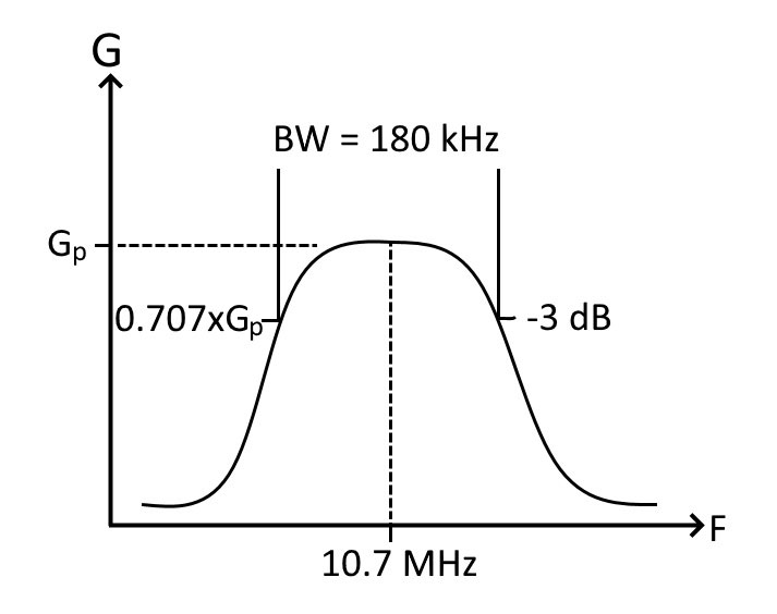
FIGURE 4. IF response curve for an FM radio.
To meet gain and response curve requirements at 10.7 MHz, FM radios need at least two IF amplifier stages with three IF transformers. Sometimes, a third IF limiter stage is included to eliminate amplitude variations in the FM signal that can pass through the FM detector as noise.
Regarding FM detectors, a brief word about their design is in order. Recall that the frequency of an FM signal varies in accordance with the frequency of the modulating audio. To extract the audio, the FM detector’s output voltage must vary in direct proportion to input frequency variation above and below the carrier frequency. Figure 5 depicts this ideal frequency-to-voltage relationship based on the FCC’s maximum allowable frequency deviation ±75 kHz and centered at the FM standard IF frequency 10.7 MHz.
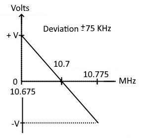
FIGURE 5. FM frequency-to-voltage conversion graph.
The actual FM detector response curve of Figure 6 combines the 180 kHz bandwidth of Figure 4 with the frequency-to-voltage relationship of Figure 5.
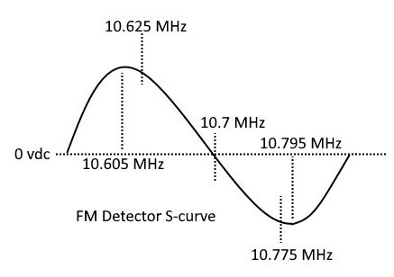
FIGURE 6. Ideal FM detector S-curve.
Because of its shape, it’s called an S-curve. An ideal IF S-curve exhibits the following characteristics: (1) balance: peak heights equal and opposite in polarity located at ±(BW/2) (±95 kHz in the example); (2) symmetry: peaks shaped the same; (3) linearity: a straight line response at least over ±75 kHz centered at 10.7 MHz (linear between the 10.625 MHz and 10.775 MHz in the example); and (4) selectivity: a rapid fall-off of response after the peaks. Several circuits produce this response curve. The two found most often in vintage radios are the discriminator and ratio detector.
Both FM detectors contain tuned circuits that must be aligned along with those in the IF amplifier. Like IF tuned circuits, their alignment involves adjusting them to resonate at 10.7 MHz. Proper alignment of the detector transformer results in an S-curve that is symmetrically peaked about zero volts at 10.7 MHz. Because the FM IF response curve is broad and flat in shape, tuning to resonance is easier said than done.
FM IF transformers are generally permeability tuned using small ferrite slugs that tend to turn in small unpredictable amounts. The result is relatively large jumps in frequency making it difficult to locate the exact center of the resonant peak. Often, even after careful adjustment, the IF response curve may not be satisfactory.
The imperfections this produces in the S-curve may not be fully realized until a listening test reveals them. Worse yet, they are not correctable without visual inspection. This brings me back to where I began: the alignment problem with my Magnavox. While I followed the service documentation’s signal generator/voltmeter alignment procedure carefully, the listening test suggested that there was still an alignment problem. This is the basis for my conclusion that visual alignment with a sweep generator and oscilloscope was the best way to align FM radios.
Tracking Alignment Basics
Vintage radios tune across a band of frequencies: 535 to 1705 kHz on AM and 88 to 108 MHz on FM. The tuned circuits meant to accomplish this must be adjusted to achieve the same level of performance across the entire band. The most often found design strategy is: (1) optimized reception at a specific frequency on the low end of the tuning dial; (2) include a way to adjust reception at a frequency on the high end of the tuning dial; and (3) mark the tuning dial at intervals where the remaining frequencies fall. The procedure that involves adjustments related to numbers (1) and (2) is called “tracking alignment.” Basically, it proceeds this way. The tuning dial is physically positioned to receive a signal at a specified frequency on the low end of the tuning dial. The frequency is sometimes specified in the service documentation. If it’s not, 600 kHz or 88 MHz work reasonably well.
Then, adjustments are made to receive a signal at a specified frequency on the upper end of the tuning dial. This frequency may be found in the service documentation. If unavailable, 1500 kHz and 108 MHz will generally work. The method of adjustment varies depending on the radio. Examples discussed shortly provide more insight into tracking procedures.
Two final notes on this subject. Occasionally, a radio will have provision for aligning the lower end of the tuning dial as well as the upper end. In such a case, following the service documentation is a must. Second, always perform IF alignment before tracking alignment. Correct tracking is based on the radio having first been aligned to a specified IF frequency.
Sweep Alignment Basics
With traditional sweep alignment, a sweep generator injects a signal at the first IF stage and the detector output is displayed on an oscilloscope as a frequency versus amplitude plot. For both AM and FM radios, IF transformers are adjusted using visual clues to obtain the desired response curve. Additionally, for FM radios, the FM detector transformer is adjusted for a satisfactory S-curve.
In actual practice, little advantage is gained using sweep alignment with AM radios. Satisfactory results can usually be obtained by simply adjusting the IF transformers to peak IF output using a signal generator/voltmeter. To increase the bandwidth in high fidelity radios and receivers, IF transformers are sometimes “stagger” tuned meaning they are peaked at frequencies slightly different from 455 kHz. In this case, visual alignment is advantageous.
Figure 7 shows a block diagram of an AM sweep alignment setup.
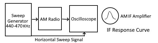
FIGURE 7. Sweep generator/oscilloscope AM alignment block diagram.
In this example, the sweep generator sweeps from 440 kHz to 470 kHz and the IF response curve is visually peaked at 455 kHz. The horizontal sweep signal synchronizes the oscilloscope time base to the sweep rate. The sweep signal is injected before the first IF stage and the AVC voltage is monitored with the vertical input of the oscilloscope. The oscilloscope displays a plot of frequency on the horizontal axis versus IF amplifier output on the vertical axis.
Figure 8 shows a block diagram of an FM sweep alignment setup.
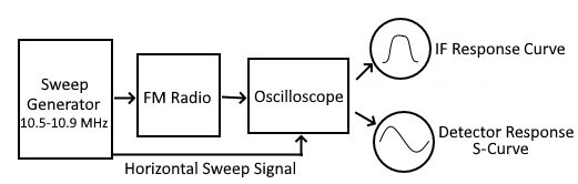
FIGURE 8. Sweep generator/oscilloscope FM alignment block diagram.
The sweep generator is configured to sweep from 10.5 to 10.9 MHz at a set rate. Using visual clues, the IF amplifier stages are tuned to obtain the desired IF response curve. The FM detector is then adjusted to obtain a satisfactory S-curve.
The oscilloscope’s vertical voltage scale can be used to determine sweep response amplitude. Frequency on the horizontal axis can’t be read directly. To address this, a “marker generator” is used to produce a small ripple or “marker” on the response curve at a preselected frequency. The marker can be positioned anywhere along the response curve to determine response curve amplitude at the preselected frequency.
While sweep alignment offers considerable advantages — particularly with FM radios — the traditional sweep generator/oscilloscope approach has a couple of weak points. First, having the use of only one marker frequency at a time can be frustrating, especially when several frequencies must be checked repeatedly during alignment. A second issue is frequency inaccuracy and drift, both commonly associated with tube model instruments. Small errors in frequency can be tolerated but frequency drift during alignment cannot be. With FM, a drift of as little as 15 kHz while adjusting IF transformers can severely affect the quality of the finished alignment. Both these problems are solved by switching from an analog to digital design.
WSAB Design and Operation
The WSAB combines sweep generator and oscilloscope functions into a single unit using modern digital technology. This not only simplifies the traditional sweep generator/oscilloscope setup, it addresses the weak points noted above. Instead of a single marker, the versatile microprocessor-controlled display can show multiple markers on the response curve at once. Frequency accuracy and drift problems disappear with digital synthesis of the sweep signal. On top of this, the cost of the WSAB is a fraction of a sweep generator/oscilloscope setup.
In the WSAB block diagram of Figure 9, a Pro Mini Arduino digitally controls the AD9850 DDS module and the TFT (Thin Film Transistor) display.
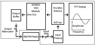
FIGURE 9. WSAB (WhippleWay Sweep Alignment Board) block diagram.
The AD9850 is a highly integrated device that uses advanced DDS technology coupled with an internal high speed/high performance D/A converter and comparator to form a complete digitally programmable frequency synthesizer. The Pro Mini communicates serially with the DDS module that, in turn, produces sine waves that sweep in small frequency steps between starting and ending frequency set points. The sweep cycle repeats approximately two times per second — slower than traditional analog sweep generators — but is still fast enough for alignment purposes.
The TFT display plots sweep amplitude versus frequency. The left edge of the display marks the starting frequency; the right edge marks the ending frequency. The starting and ending frequencies are chosen to cover just beyond the response curve limits of the IF amplifier. The sweep center is the specified IF frequency, 455 kHz or 10.7 MHz. The TFT display also serves along with two rotary encoders and two pushbuttons as a user interface to determine sweep mode and to modify operational parameters.
Two analog circuits complete the design. The sweep output circuit uses a common emitter transistor circuit to buffer the AD9850 output. A selector switch provides course output level control and a potentiometer for fine control. The sweep input circuit consists of a potentiometer input gain control followed by a precision operational amplifier, a TLE 2021. Besides providing a gain of 2, the op-amp circuitry functions with the Pro Mini to control the plotted polarity and range.
Circuit Design Details
Figure 10 shows the sweep output circuitry.
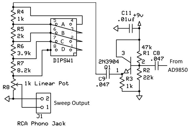
FIGURE 10. WSAB sweep output circuit diagram.
Sine wave output from the AD9850 feeds an emitter-follower transistor that provides a low impedance output to the attenuation circuit consisting of resistors R4 to R7 and potentiometer R8, the Sweep Output Level control. DIP switches S1A to S1D provide course output attenuation of 1/2, 1/4, 1/8, and 1/16. Potentiometer R8 then provides fine attenuation control. The sweep input circuit must handle input voltages that are positive, negative, or both for an S-curve.
The range accommodated for tube radios is ±8 volts. Since the analog input of the Pro Mini is restricted to zero to five volts, the sweep input circuitry must translate -8 to +8 volts to 0 to 5 volts. The circuit in Figure 11 does the job.
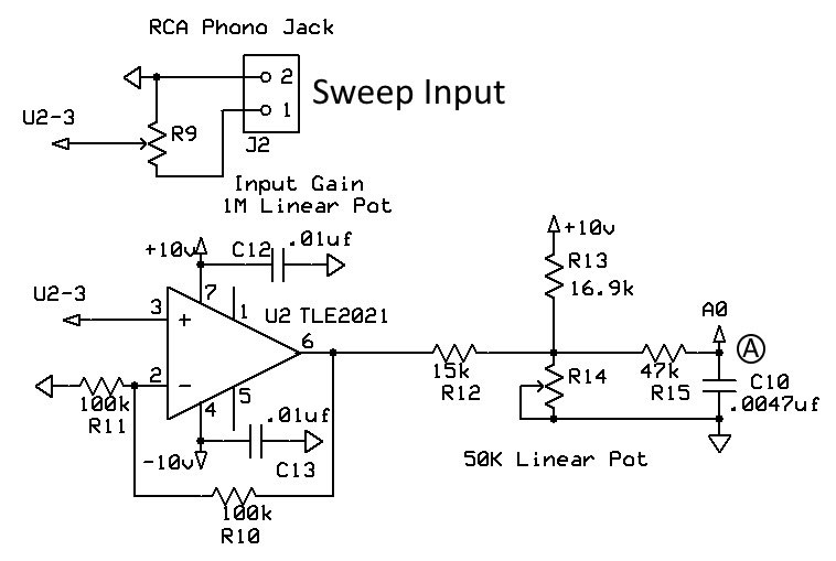
FIGURE 11. WSAB sweep input circuit diagram.
The heart of the circuit is an op-amp with a voltage gain of 2, preceded by potentiometer R9 acting as the Sweep Input Gain control. The combination of resistors R12, R13, and R14 shifts and attenuates the op-amp’s ±8 volts output to 0 to 5 volts. Potentiometer R14 is used to set 2.5 volts at point “A” when sweep input is zero. Resistor R15 and capacitor C10 provide noise and RF/IF signal filtering prior to the Pro Mini analog input A0.
To handle the op-amp’s ±8 volts range, a ±10 supply voltage was needed. Because the supply current was very small, a MAX680 charge pump IC was chosen to supply the ±10 volts. Refer to Figure 12.
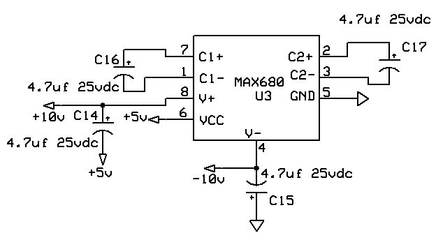
FIGURE 12. WSAB charge pump plus/minus power supply circuit diagram.
The five volts required to power the Arduino Pro Mini, the AD9850 module, MAX680, and TFT display is supplied by a nine volt DC wall adapter and an LM7805 voltage regulator IC as shown in Figure 13.
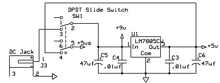
FIGURE 13. WSAB five volt power supply circuit diagram.
Besides performing the on-off function, switch SW1 also isolates the Pro Mini in the off position so that it can be programmed from a PC. The Pro Mini interconnections with the AD9850 and display are shown in Figure 14.
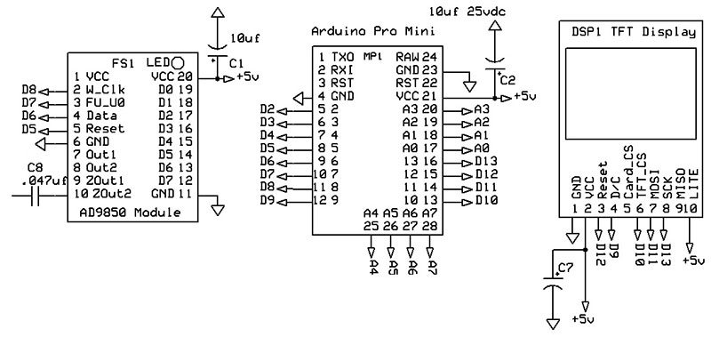
FIGURE 14. WSAB Pro Mini, AD9850 module, and TFT display circuit diagram.
Pro Mini digital inputs and outputs provide a serial communication link with the AD9850 and TFT display. Lastly, two buttons and two rotary encoders round out the design as in Figure 15.
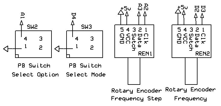
FIGURE 15. WSAB pushbutton and rotary encoder circuit diagram.
All digital I/O bits on the Pro Mini are used, so I had to enlist the use of analog inputs A1, A2, and A3 to serve a digital function.
The complete schematic is shown in Figure 16.
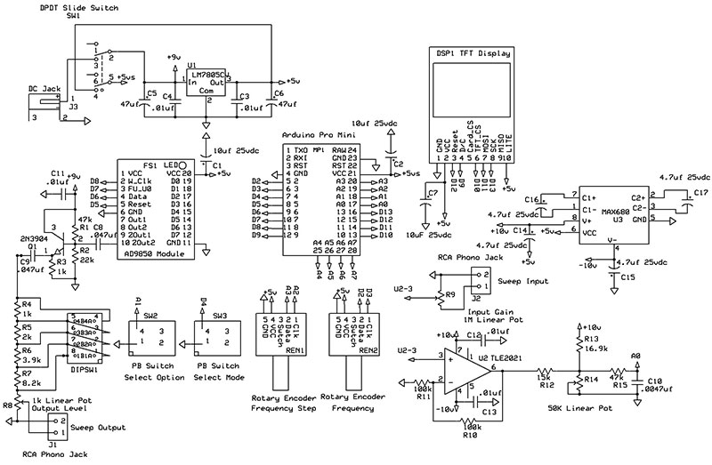
FIGURE 16. WSAB complete circuit diagram.
A graphics (BMP) file of the schematic is available with the downloads for this article.
Interpreting the WSAB Display
Because the small 1.8“ display has a limited number of characters on a line, I had to use abbreviations and, in some cases, omit measurement units altogether.
Figure 17 shows a sample response curve from an AM IF amplifier.
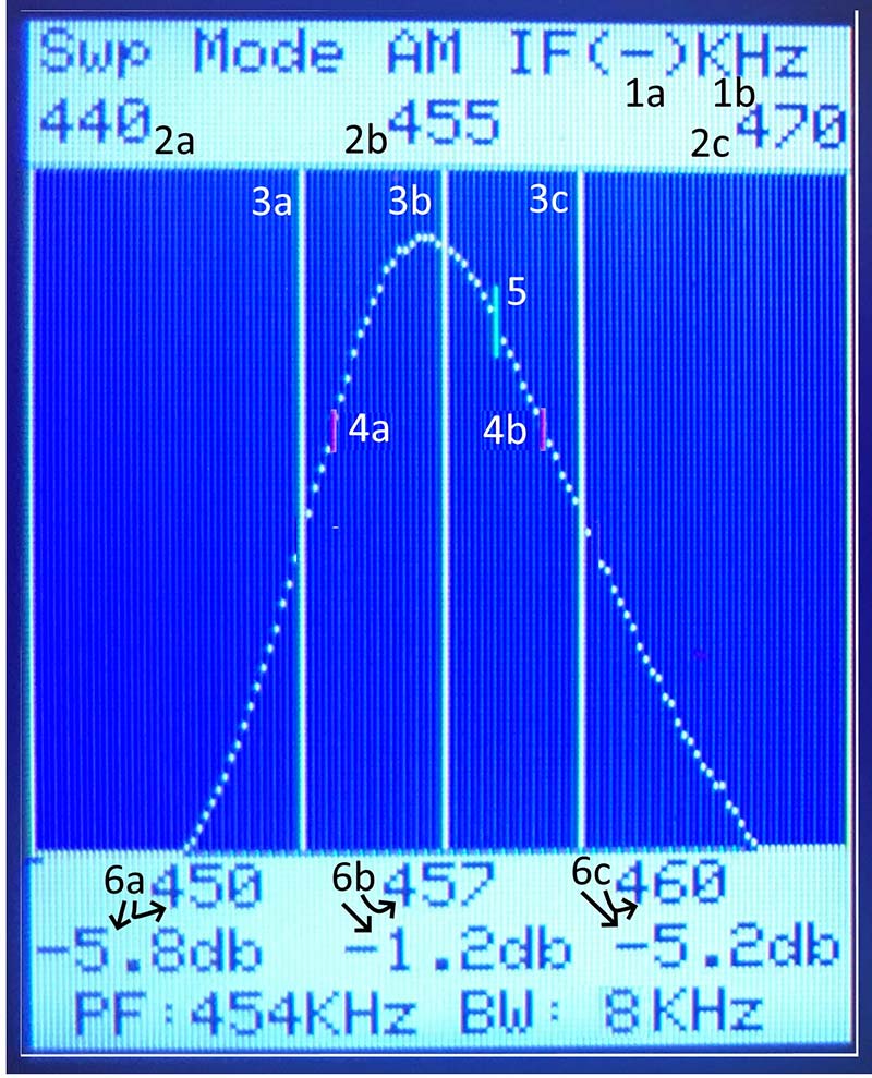
FIGURE 17. AM IF sweep response with annotations.
The selected sweep mode “Swp Mode” appears on the first line and is one of the following:
Mode 0 “AM IF (-) kHz” – AM IF alignment. 455 kHz center frequency. Displays negative input voltage from the bottom of the plot area. Most tube type AM radios use this mode.
Mode 1 “AM IF (+) kHz” – AM IF alignment. 455 kHz center frequency. Displays positive input voltage from the bottom of the plot area. Transistor radios sometimes use this mode.
Mode 2 “FM IF (-) MHz” – FM IF alignment. 10.7 MHz center frequency. Displays negative input voltage from the bottom of the plot area. Used for FM IF alignment.
Mode 3 “FM IF (+) MHz” – FM IF alignment. 10.7 MHz center frequency. Displays positive input voltage from the bottom of the plot area. Used for FM IF alignment.
Mode 4 “FM SS (±) MHz” – FM detector alignment. Displays a single S-curve (SS) centered at 10.7 MHz. FM radios use this mode to align the S-curve.
Mode 5 “FM DS (±) MHz” – FM detector alignment. Displays a double S-curve (DS) centered at 10.7 MHz. One is the normal S-curve as in Mode 4. The other is an image of the S-curve reversed and inverted. The resulting double S-curve is handy for checking S-curve balance and symmetry.
For the remaining items, refer to the reference numbers in Figure 17.
1a. The polarity of the input for the displayed plot: (-) negative up with zero volts at the bottom of the plot area; (+) positive up with zero volts at the bottom of the plot area; and (±) both positive (up) and negative (down) with zero volts at the vertical center of the plot area. Example: (-) negative up with zero volts at the bottom of the plot area.
1b. The default frequency units for the display, either kHz or MHz. Used when the frequency unit is omitted. Example: Default frequency is kHz.
2a. The starting frequency of the sweep. Example: 440 kHz.
2b. The center frequency of the sweep. Example: 455 kHz.
2c. The ending frequency of the sweep. Example: 470 kHz.
3a. The Lower Frequency Marker line indicating frequency 6a below. Example: 450 kHz.
3b. The Center Frequency Marker line indicating frequency 2b above. Example: 455 kHz.
3c. The Upper Frequency Marker line indicating frequency 6c below. Example: 460 kHz.
4a. The Lower Bandwidth Marker for voltage gain of -3 dB based on the peak frequency amplitude.
4b. The Upper Bandwidth Marker for a voltage gain of -3 dB based on the peak frequency amplitude.
5. The Variable Frequency Marker indicating frequency 6b below. This frequency is adjustable using the Frequency Step and Frequency controls. Example: 457 kHz.
6a. The Lower Frequency Marker voltage gain at the stated frequency based on the peak frequency voltage. Example: -5.8 dB at 450 kHz.
6b. The Variable Frequency Marker voltage gain at the stated frequency based on the peak frequency voltage. Example: -1.2 dB at 457 kHz.
6c. The Upper Frequency Marker voltage gain at the stated frequency based on the peak frequency voltage. Example: -5.2 dB at 460 kHz.
PF. The frequency of the peak amplitude. Example: 454 kHz.
BW. The bandwidth of the sweep at -3 dB frequencies, 4a and 4b. Example: 8 kHz.
Operational Controls
Figure 18 shows the six controls used to operate the WSAB.
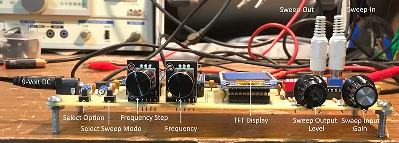
FIGURE 18. WSAB operational controls.
The function of each control is described next. Note: “Example” refers to the response curve of Figure 17.
1. Select Option Button – Press the Select Option button to cycle through operational parameters “a” to “d” below. When an operational parameter is selected, use the Frequency Step and Frequency Controls to change its value.
a. Change Center Frequency of scan. Example: 455 kHz.
b. Change Width of Scan (ending sweep frequency/starting sweep frequency). Example: 30 kHz (440 kHz to 470 kHz, 15 kHz either side of 455 kHz).
c. Change Lower Marker. The frequency of the marker line below the center frequency. Example: 450 kHz.
d. Change Upper Marker. The frequency of the marker line above the center frequency. Example: 460 kHz.
2. Mode Option Button – Press the Mode Option button to cycle through the sweep modes “0” to “5” below.
Mode 0: “AM IF (-) kHz” – AM IF alignment. 455 kHz center frequency. Displays negative input voltages.
Mode 1: “AM IF (+) kHz” – AM IF alignment. 455 kHz center frequency. Displays positive input voltages.
Mode 2: “FM IF (-) MHz” – FM IF alignment. 10.7 MHz center frequency. Displays negative input voltages.
Mode 3: “FM IF (+) MHz” – FM IF alignment. 10.7 MHz center frequency. Displays positive input voltages.
Mode 4: “FM SS (±) MHz” – FM detector alignment. Single Sweep 10.7 center frequency. Displays positive/negative voltages.
Mode 5: “FM DS (±) MHz” – FM detector alignment. Double Sweep 10.7 center frequency. Displays positive/negative voltages.
Note: On power-up, the sweep mode is “AM IF (-).” Pressing the Select Mode button rotates through the other modes. Pressing the Select Option button in any sweep mode cycles through the mode’s operational parameters, each of which can be changed using the Frequency Step and Frequency Controls.
3. Frequency Controls – Use these controls to change an operational parameter. (See item 1 above.)
Frequency Step Control: Rotate the Frequency Step Control to select the step size used with the Frequency Control. Steps range from 1 kHz to 5 MHz.
Frequency Control: Rotate the Frequency Control clockwise to increase or counterclockwise to decrease the operational parameter’s frequency by the Frequency Step size selected.
Note: When in Sweep Mode, the frequency controls change the Variable Frequency Marker (6b in the sample response curve in Figure 17). This feature permits inspecting response curve amplitude at any frequency between the starting and ending frequencies.
4. Sweep Output Level – Use this control to vary the level of sweep output from 0 to ~100 millivolts. The maximum output level can be reduced using the DIP switch attenuator (DIPSW1) that provides scaled output reductions of 1/2, 1/4, 1/8, and 1/16.
5. Sweep Input Gain – Use this control to vary the sweep input gain. Fully clockwise is a gain of 2 with maximum peak-to-peak voltage of approximately eight volts.
Building the WSAB
The WSAB ExpressPCB schematic and printed circuit board (PCB) files are available in the article downloads. Figure 19 is the WSAB PCB.
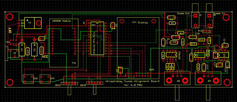
FIGURE 19. WSAB printed circuit board.
All components are through hole and most are available from Jameco. A few specialized components are available from other sources. See the Parts List for purchasing information for all parts.
Use DIP sockets for the AD9850 module, the Pro Mini, the TLE2021 op-amp, the MAX680 charge pump, and the TFT display.
The Pro Mini uses a wide (0.6 in) 24-pin DIP socket; Jameco 112264. The TLE2021 and MAX 680 use an eight-pin DIP socket; Jameco 112206.
The AD9850 module and TFT are non-standard and are easily accommodated by cutting two 20-pin DIP sockets (Jameco 112248) in half. The AD9850 requires two 20-pin halves and the TFT display requires one.
Figure 20 shows the completed unit.
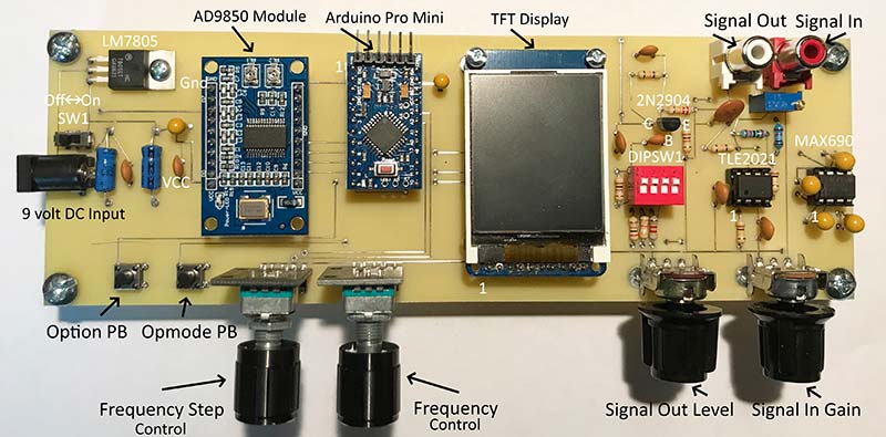
FIGURE 20. Completed WSAB PCB.
No case is provided. Instead, use four no. 8 x 3/4” machine screws and nuts in the corners of the PCB to serve as feet. Use four no. 4 x 3/4” machine screws and nuts supporting the upper edge of the TFT display (the edge opposite the connecting pins).
Place one nut above the PCB and one below, then adjust their positions so that the TFT display is parallel to the PCB. Finally, use a no. 6 x 1/4” machine screw and nut to mount the LM7805 regulator.
To make the sweep input and output cables, sacrifice an RCA male-to-male audio cable and two mini-clip leads. Cut each in two. If necessary, trim the audio cable lengths to 10 inches and the clip lead lengths to three inches. Splice and solder as shown in Figure 21.
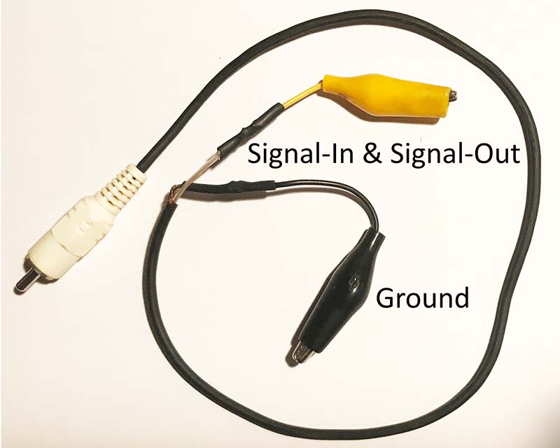
FIGURE 21. Construction of WSAB input and output cables.
Use heat shrink tubing to strengthen the splices.
WSAB Arduino Code
The library and program code used in the WSAB project are available in the downloads. The code is broken down into two major sections: the first handles the five sweep modes while the second takes care of modifying operational parameter values. Changes and additions are readily accomplished including the addition of other sweep modes (IF frequency and plot polarity).
It’s assumed that the user is familiar with Arduino programming. The SparkFun FTDI Basic Breakout 5V programming tool or similar is needed to program the Pro Mini. Pro Minis are available from several sources and may differ in the order of programming pins. Compare the female pins on the FTDI board with the male pins on the Pro Mini to make sure the VCC (5V) pins line up. Experience has shown that orientation can be either FTDI component side up or down depending on the purchase source of the Pro Mini. When the WSAB’s power switch is turned off, the internal five volt supply is disconnected from the Pro Mini, so the programming tool can be safely connected for programming.
Initial Power-Up Procedure
Start with the bare board, i.e., no devices plugged in.
- With the power switch (S1) in the OFF position, attach the nine volt DC supply. Turn WSAB power on and check that the VCC marked pin of the AD9850 is five volts. Turn power off.
- Plug in U3, the MAX680. Observe the location of pin 1. Turn power on and check that pin 4 of U2, the TLE2021, is -10 volts and pin 7 is +10 volts. Turn power off.
- Plug in U2, the TLE2021. Observe the location of pin 1. Clip signal-in to signal-in ground. Turn power on. Adjust trimmer R14 for 2.5 volts at the junction of R15 and C10 (point A in Figure 11). Turn power off.
- Plug in the remaining devices. Observe that the VCC pin on the AD9850 appears next to the VCC marked on the PCB. Observe that the programming pins of the Pro Mini face the back of the PCB. The TFT display can be plugged in only one way.
- Turn power on. In a few seconds, the TFT display will show the screen for Mode 0: AM IF(-) kHz.
- Use an AM radio to check that the DM9850 is functioning. Tune the radio to 910 kHz, the second harmonic of 455 kHz. With the WSAB close to the radio, a thumping sound should be heard as the WSAB sweeps past 910 kHz.
- Press the Sweep Mode button repeatedly until Mode 4 “FM SS (±) MHz” shows. With the signal-in still clipped to signal-in ground, adjust trimmer R14 in both directions. The horizontal signal line should move above and below the horizontal center line. Leave it exactly on the line.
- Unclip the signal-in from the signal-in ground. Turn the Signal Sweep Input control fully clockwise (full gain). Hold the signal-in between your fingers; 60 Hz line noise should be visible on the TFT display indicating the signal-in circuit is functioning correctly.
- Press the Select Option button once to get the Set Center Frequency option. Use the Frequency Step and Frequency Control to change the center frequency to a convenient frequency on the AM broadcast band. Tune the radio to that frequency and listen for the signal. Since the WSAB signal is unmodulated, listen for changes in the noise level. Move the center frequency above and below by small frequency steps to be certain the WSAB signal is that received.
Wrap-Up
The preceding steps exercise most of the WSAB’s basic functions but for a true test, an actual alignment would be best. AM alignment is a good place to try first since it’s simpler than FM. That will be the starting point for Part 2 of this series.
I’ll cover basic sweep alignment procedures for AM and FM radios plus an actual example of each. Stay tuned! NV
Parts List
| Part |
Description |
Source |
| C1 |
10 µF 25 VDC |
Jameco 94060 |
| C2 |
10 µF 25 VDC |
Jameco 94060 |
| C3 |
.01 µF |
Jameco 15229 |
| C4 |
.01 µF |
Jameco 15229 |
| C5 |
47 µF |
Jameco 135319 |
| C6 |
47 µF |
Jameco 135319 |
| C7 |
10 µF 25 VDC |
Jameco 94060 |
| C8 |
.047 µF |
Jameco 15253 |
| C9 |
.047 µF |
Jameco 15253 |
| C10 |
.0047 µF |
Jameco 15211 |
| C11 |
.01 µF |
Jameco 15229 |
| C12 |
.01 µF |
Jameco 15229 |
| C13 |
.01 µF |
Jameco 15229 |
| C14 |
4.7 µF 25 VDC |
Jameco 546071 |
| C15 |
4.7 µF 25 VDC |
Jameco 546071 |
| C16 |
4.7 µF 25 VDC |
Jameco 546071 |
| C17 |
4.7 µF 25 VDC |
Jameco 546071 |
| DIPSW1 |
|
Jameco 696950 |
| DSP1 |
TFT Display |
Amazon DSD TECH 1.8 inch TFT |
| FS1 |
AD9850 Module |
Amazon HiLetgo DDS AD9850 |
| J1 |
RCA Phono Jack |
Mouser 806-KLPX-0848-2-W |
| J2 |
RCA Phono Jack |
Mouser 806-KLPX-0848-2-W |
| J3 |
DC Jack |
Jameco 2210677 |
| MP1 |
Arduino Pro Mini |
|
| Q1 |
2N3904 |
Jameco 38359 |
| R1 |
47K |
Jameco 691260 |
| R2 |
22K |
Jameco 691180 |
| R3 |
1K |
Jameco 690865 |
| R4 |
1K |
Jameco 690865 |
| R5 |
2K |
Jameco 690937 |
| R6 |
3.9K |
Jameco 691008 |
| R7 |
8.2K |
Jameco 691083 |
| R8 |
1K Linear Pot |
Jameco 2271663 |
| R9 |
1M Linear Pot |
Jameco 2271679 |
| R10 |
100K |
Jameco 691340 |
| R11 |
100K |
Jameco 691340 |
| R12 |
15K |
Mouser 660-MF1/4CCT52R1502F |
| R13 |
16.9K |
Mouser 660-MF1/4CC1692F |
| R14 |
50K Linear Pot |
Jameco 853791 |
| R15 |
47K |
Jameco 691260 |
| REN1 |
Rotary Encoder |
Amazon Cylewet KY-040 |
| REN2 |
Rotary Encoder |
Amazon Cylewet KY-040 |
| SW1 |
DPDT Slide Switch |
Jameco 161817 |
| SW2 |
PB Switch |
Jameco 149948 |
| SW3 |
PB Switch |
Jameco 149948 |
| U1 |
LM7805CV |
Jameco 51262 |
| U2 |
TLE2021 |
Mouser 595-TLE2021CPE4 |
| U3 |
MAX680 |
Mouser 700-MAX680CPA |
Downloads
What’s In The Zip?
Complete Schematic
ExpressPCB Schematic and PCB Files
Library and Program Code
Rotary-Master Zip File
TFT-Master Zip File