In about 10 minutes and for about $6, you can display the blood flow through your finger, like the plot in Figure 1.
From this measurement, you can extract your heart rate, check for arrhythmia, and even modulate a red light to pulsate with your heart rate. Here’s how.
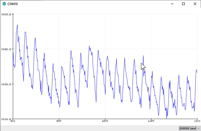
FIGURE 1. An example of the measured output of this PPG instrument showing the blood flow through my finger.
The Method
The method we’ll use which measures the changes in the reflected light from the blood flowing in your finger is called photoplethysmogram, or PPG. This term translates to using light to measure volume changes of an organ; in this case, blood.
This is the same technique your Fitbit or iWatch uses to track your heart rate. We shine an LED into your finger and measure the reflected light intensity. From the changes in the light coming back to the detector, we interpret your blood flow. This method uses reflected, or scattered light, rather than transmitted light. It just makes it easier to implement since we don’t need access to both sides of your finger. In principle, we could apply this technique to any part of your body in which blood is flowing. Your finger is the most convenient.
When more blood is in your finger, we get more scattered light back to the detector. When less blood flows, we get less scattered light. The problem is this is a very small effect, so we need to do a few special tricks to see this small signal in the presence of a lot of noise.
In addition, we want the absolute simplest, easiest to use, and easiest to set up sensor, so we’ll do all the signal processing in the few lines of code we write.
To implement a PPG instrument, all it takes is an ultra-bright red LED, a photo-sensitive resistor (PSR), and an Arduino. The total cost including the Arduino is about $6; less if you have any of these three items already.
There is no wiring required, no fixtures; just plug the components in, write the sketch, put your finger on top of the sensor, and see your pulse.
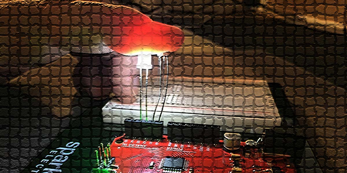
It doesn’t get any easier, faster, or cheaper than this. That’s why I call this an Instant Heart Pulse Sensor. The entire system — complete with finger attached — is shown in Figure 2.
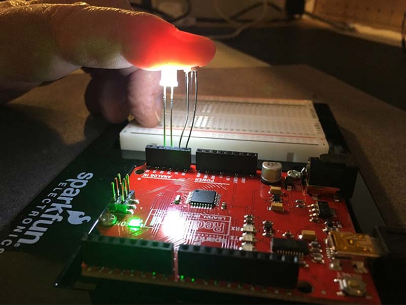
FIGURE 2. The complete system of Arduino, LED, photo-sensitive resistor, and finger measuring my PPG signature.
To make this so simple, we’re going to violate a few general guidelines for using the Arduino Uno board and use six little known tricks.
Trick #1: Analog Pins are Really GPIO Pins
On the Arduino Uno, there are digital I/O pins labeled D13 to D0, and analog pins labeled as A0 to A5. Figure 3 shows the analog pins on a common Uno board. If you don’t have an Arduino board, you can purchase one from SparkFun for about $20 or from AliExpress for about $4.
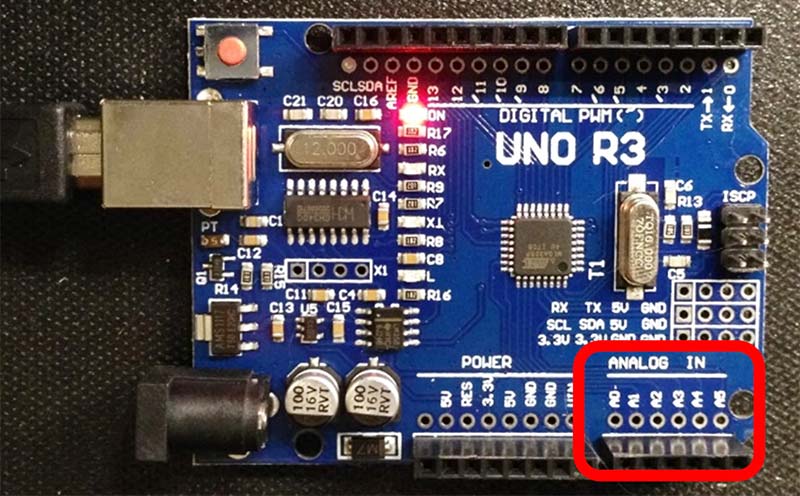
FIGURE 3. The Arduino Uno with the analog pins in the lower right of the board, identified by the square.
While these pins are labeled as analog pins, they are really “anything” pins. They can be configured as digital input, digital output, and analog input pins. They are called general-purpose I/O pins or GPIO pins. We’ll use two of the analog pins to power the LED.
We set these two adjacent pins as digital pins for OUTPUT. One we set HIGH and the other we set LOW. This effectively connects the 5V Vcc voltage on the HIGH pin and ground on the LOW pin.
The connections to these power and ground rails are through the output transistors of the pins. The pins themselves add about 80 ohms of internal resistance in the circuit.
Trick #2: Direct Drive an LED with the Output Pin of an Arduino
Every manual or project guide you read will tell you don’t stick an LED directly into an Arduino’s digital I/O pins. Always add a current-limiting series resistor. While you should not stick an LED between the 5V power rail and ground — or it will die a quick and rather unspectacular death — plugging it directly into an Arduino digital pin is not so bad.
Even though the HIGH and LOW pins are connected to 5V and ground, respectively, there is really about 40 ohms of resistance in each pin path. This means when you plug a red LED between these two pins, the 80 ohm resistance in the output transistors of the pins themselves will limit the current. With a 2V drop across the LED, the voltage across the internal resistance is about 3V. This means the current will be about 3V/80 ohms = 38 mA.
While this is a high current for an LED, we want a lot of current to make a very bright LED. Running even 40 mA through an LED will not harm the Arduino or the LED. The LED may not last 10 years and may burn out in a few months, but they cost less than five cents each. We’re hackers. It’s worth it.
I like using the Arduino Uno board (which at its heart is the ATmega 328 microcontroller) because its outputs can source and sink more than 40 mA of current. This is plenty to drive an ultra-bright LED. Other Arduino boards — like the ones based on a SAMD21 microcontroller — are great boards, but can only source and sink about 7 mA of current. When we plug an LED directly into these pins, the LED will turn on with about 38 mA of current flowing through it. Just be cautious! When you drive 38 mA of current through an ultra-bright LED, the light can be VERY bright. Do not stare directly into the LED.
In this example, I’m setting pin A0 as HIGH and pin A1 as LOW. The entire sketch to drive the LED is just a few lines:
void setup() {
pinMode(A0, OUTPUT);
pinMode(A1, OUTPUT);
digitalWrite(A0, HIGH);
digitalWrite(A1, LOW);
}
void loop() {
}
The LED’s anode pin goes into A0 and the cathode lead; the short lead, or the lead next to the flat in the flange, goes into the A1 pin.
If you have a selection of LEDs and can’t tell what color they are or how bright they are, you can use this simple setup to test them out. Just plug a candidate LED into the A0 and A1 pins and you will instantly see what color it is and how bright it is. Figure 4 shows an example of a red LED in these two pins.
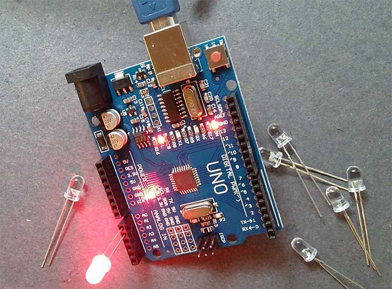
FIGURE 4. An example of an LED in pins A0 and A1.
In principle, you can use any color LED for PPG. Since your blood looks red, this means it absorbs all the other colors except red and scatters red the most. This makes it a good color to select. However, there’s a balance between the brightest red you can find and the brightest of another color or white LED you can find and the peak sensitivity of the detector, which is actually green at 540 nm. You should try experimenting with other color LEDs to see which is the most sensitive for your PPG.
If you don’t have any ultra-bright LEDs, you can purchase 100 of them for about $8 on Amazon, or a similar assortment of LEDs for $2 on AliExpress.
Trick #3: Use a Pull-up Resistor On a Digital I/O to Bias the Photoresistor
The photo sensor we’ll use is a simple photoresistor. It has a nominal resistance of about 200K ohms in the dark and drops its resistance to about 3K when light falls on it. The resistance of the sensor is directly related to the light intensity that falls on the sensor, though in a very non-linear way. Figure 5 shows an example of a photosensitive resistor (PSR).
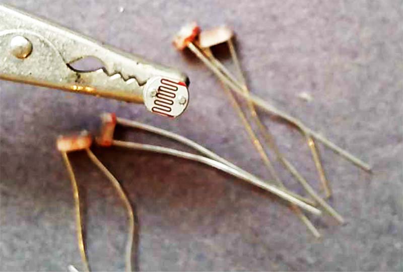
FIGURE 5. Close-up of a PSR.
There are a range of PSRs available, each with a different part number. Their response times are all about 30 msec. Their peak wavelength of sensitivity is all the same; 540 nm which is green. However, they differ in their light and dark resistance. Table 1 shows a summary of the resistance ranges for the different parts from their spec sheets.
| Part Number |
Light Resistance |
Dark Resistance |
| 5506 |
6K |
150K |
| 5516 |
10K |
200K |
| 5526 |
20K |
1M |
| 5528 |
20K |
1M |
| 5537 |
50K |
2M |
| 5539 |
90K |
5M |
| 5549 |
140K |
10M |
TABLE 1.
The sweet spot for using this trick to measure the resistance of the PSR is for a dark resistance less than 1M. If you have a choice, select a PSR that has a low dark resistance. If you don’t know the type of PSR you have, that’s okay. You can measure it and see if it works. The methods introduced here are pretty robust, so just about any PSR might work.
If you don’t have one of these PSRs laying around, you can purchase a pack of 50 of them with a range of part numbers for about $6 from Amazon, or 50 of them for $1 from AliExpress.
The Arduino ADC (analog-to-digital converter) pins can only measure a voltage. To measure the resistance of the PSR, we need to turn the resistance into a voltage. We do this using a simple voltage divider circuit. It’s literally as simple as using a voltage source and resistor in series with the PSR.
We measure the voltage on the PSR and from the voltage of the pin set for HIGH, we can calculate the resistance of the PSR. The voltage divider circuit is shown in Figure 6.
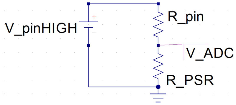
FIGURE 6. A simple voltage divider circuit.
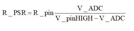
In this circuit, the voltage measured by the ADC is:
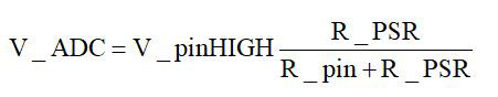
With a little algebra, the resistance of the PSR sensor is:
We use a not very well known trick of the GPIO pins to turn an analog pin into the front half of a voltage divider. We set the analog pin as a digital input pull-up I/O pin. This will make the digital pin be an input with a roughly 40K ohms pull-up resistor tied to the 5V rail. All we have to do is connect the PSR between this pull-up resistor and an adjacent pin, A3, set as LOW. This builds the complete voltage divider circuit.
In this example, I’m going to use analog pin A2 as the digital INPUT_PULLUP. After I set this A2 pin as an INPUT_PULLUP, I’m going to read the voltage on this A2 pin. Pin A3, set as LOW, is connected to ground through the 40 ohm pin resistance. When the PSR is connected between pins A2 and A3, the voltage on A2 will be directly related to the PSR resistance.
To translate the voltage on pin A2 into the resistance of the PSR, we need to know the internal pin voltage and the output resistance of the pin. Since we’re not trying to do accurate absolute measurements of the resistance, an approximate calibration is all we need to do. To measure the internal pin voltage, we just measure the voltage on the analog pin A2 with nothing connected. Since this is a 10-bit ADC, the measured voltage on pin A2 is:
Vmeas = ADC_ADU / 1023.0 x 5.0V
where ADC_ADU is the bit value in analog-to-digital units (ADU). The complete sketch so far is shown here:
float V_meas;
float V_internal;
float R_pin;
void setup() {
pinMode(A0, OUTPUT);
pinMode(A1, OUTPUT);
pinMode(A2, INPUT_PULLUP);
pinMode(A3, OUTPUT);
digitalWrite(A0, HIGH);
digitalWrite(A1, LOW);
digitalWrite(A3, LOW);
Serial.begin(2000000);
}
void loop() {
V_meas = analogRead(A2)/1023.0*5.0;
Serial.println(V_meas,3);
}
In this sketch, I initialize a few variables we’ll use. Then, I set the pinModes for the various pins. Next, I set the baud rate for the serial printer as 2000000. Why this high? Because the USB interface will operate this fast and faster is always better — if it’s robust. It’s just important that the serial monitor also be set for this rate. Using this sketch, I measured the voltage on pin A2 with nothing plugged in as 4.99V. This is the internal pin voltage.
To get the output pin resistance, we can do another simple trick. If we add a known resistor in place of the PSR and measure the voltage across it, we can back out the internal pin resistance as:
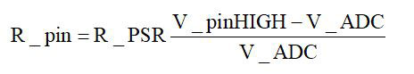
In this example, I added a 47K resistor as the R_PSR and measured a V_ADC = 2.76V. This makes the internal pin resistance:
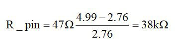
Now that we know the pin voltage and the pin resistance, we can measure the ADC voltage and know the resistance of the PSR. These values go into the initialization of the variables at the beginning of the sketch.
By measuring the voltage on the A2 ADC, we basically have a fast ohmmeter. We can estimate the resistance range to which this ohmmeter is sensitive based on the highest and lowest voltage we can measure. I use as an estimate of the highest voltage to be two bit levels or 10 mV, below the 4.99V level, or 4.98V.
The lowest voltage I can measure, I likewise estimate to be 10 mV above 0. This sets the limits to the highest and lowest resistance I can measure as:
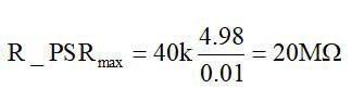
And
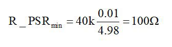
This is a pretty good dynamic range — well within the range for most PSRs we might use. Now we’re ready to measure the resistance of the PSR.
Trick #4: Average Over n Power Line Cycles to Get Lower Noise
At this point, we’re letting the ADC measure the voltage on A2 as quickly as it can, which is about every 112 µsec. It’s giving us a data point slower than this due to the print statement in the loop. This is too fast to see the data, and we see all the digitizing noise.
We could add a delay() statement to slow down the data reporting, but this wastes a lot of measurement opportunity. Instead, we’re going to average the data over a long time interval.
We can average using one of two methods: average n consecutive points using a for loop or average for a specific time interval using a while loop. The simplest is with a for loop. However, it would be nice to keep track of the time per point, and, whenever we’re measuring small signals — especially with a relatively high input resistance, >10K ohms — we’ll always have a little 60 Hz pick-up unless we’re careful.
If we average for an integral number of 60 Hz power line cycles, we will dramatically reduce the 60 Hz noise we pick up. This is called digital filtering. One power line cycle is 1/60 = 16.7 msec; two power line cycles is 2 x 16.7 msec = 33.4 nsec; and three power line cycles is 50 msec. The code to average for a fixed time is a little more involved than a simple for loop, but is still easy to implement.
The algorithm is:
√ Start a timer.
√ Add together consecutive ADC readings.
√ Run a counter to keep track of how many measurements we’re adding together.
√ Do the measurements until the timer has advanced longer than the averaging interval we set.
√ Stop the measurements.
√ Divide the running sum by the number of samples.
My sketch that implements this along with the rest of the code is:
float V_meas;
float V_internal = 4.99;
float R_pin = 38000.0;
float R_PSR;
long iTime_ave_usec = 1.0 / 60 * 1e6;
long iCounter;
long iTime0_usec;
void setup() {
pinMode(A0, OUTPUT);
pinMode(A1, OUTPUT);
pinMode(A2, INPUT_PULLUP);
pinMode(A3, OUTPUT);
digitalWrite(A0, HIGH);
digitalWrite(A1, LOW);
digitalWrite(A3, LOW);
Serial.begin(2000000);
}
void loop() {
V_meas = 0.0;
iCounter = 0;
iTime0_usec = micros();
while ((micros() - iTime0_usec) < iTime_ave_usec) {
V_meas = analogRead(A2) / 1023.0 * 5.0 + V_meas;
iCounter++;
}
V_meas = V_meas / iCounter;
R_PSR = R_pin * V_meas / (V_internal - V_meas);
Serial.println(R_PSR, 3);
}
In this sketch, I used variable names that are self-documenting and have their units with the variable name. This makes their instant interpretation so much easier.
Whenever you’re doing a measurement with a new instrument — especially one you construct yourself — it’s always valuable to measure something you know first. This way, you can get a rough idea of the accuracy and the noise of the instrument.
We have basically built a precision ohmmeter. We measure the resistance of the device between the A2 and A3 pins of the Arduino. We anticipate the range of the PSR to be about 3K to 100K ohms. How well can we measure this resistance, and how much noise or fluctuations will we get if we have a known constant resistance?
This is easy to test by inserting a simple resistor. I used the same 47K ohm resistor I used for the calibration. Figure 7 is the Arduino with the LED and the 47K resistor.
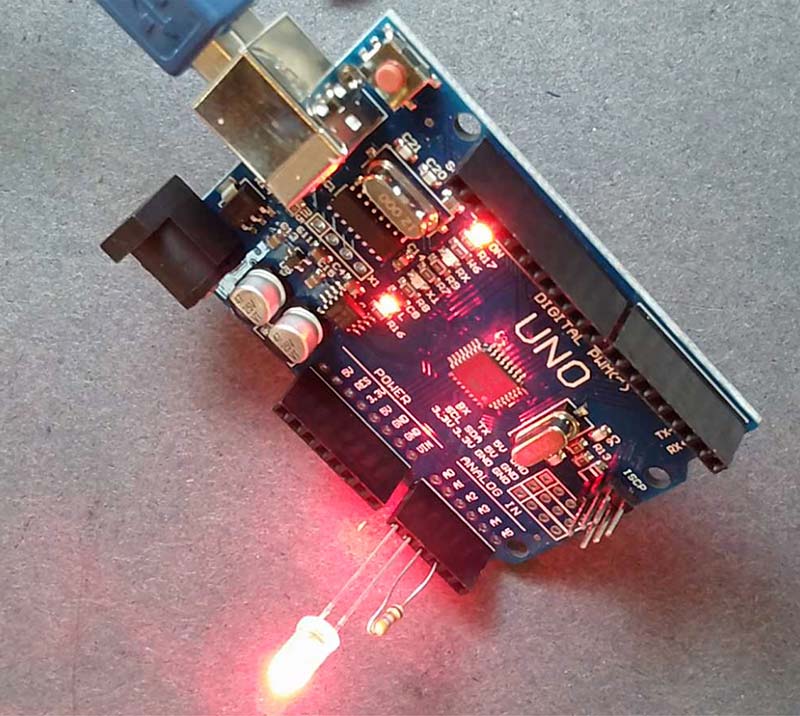
FIGURE 7. Calibration resistor plugged into pins A2 and A3.
I also used an integration time of three power line cycles or about 50 msec per point. Instead of printing the data every 50 msec onto the serial monitor, I used the serial plotter. Figure 8 is an example of a typical measurement of the resistance plotted over 500 points. This is a total time interval of about 25 sec.
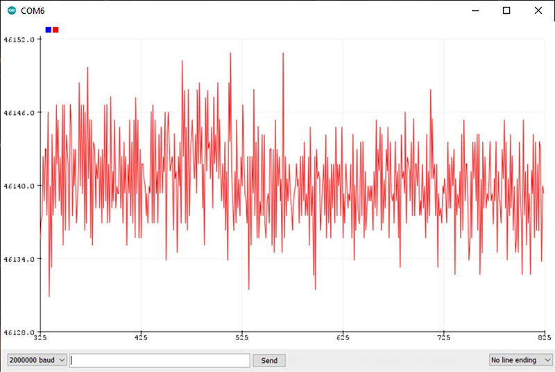
FIGURE 8. The measured resistance of the 47K ohm resistor over a 20 sec interval, with a range of six ohms per division.
This measurement shows the average value of about 46.1K ohms resistance — right what we expected — and the measurement noise of about 20 ohms peak-to-peak. This is about 0.02%. It’s basically the result of averaging the digitizing noise. This is a case where some noise in the measurement above the least bit level actually reduces the averaged noise.
This system behaves just as we expected. Now it’s time to test out our PPG.
Trick #5: Plotting On Scales You Can Adjust
The serial plotter built into the Arduino IDE (integrated development environment) is a very powerful tool. It gives a visual picture of your measurements as they come out. The horizontal scale will always be 500 points across. As new data after the 500th point comes in, the rest of the data will shift to the left, always displaying the latest 500 points.
One limitation is that the vertical scale will auto scale based on the 500 points displayed. Sometimes, I like having a fixed scale that doesn’t change. This way, I can immediately see the absolute changes or values of the data. Here’s the trick to keep the vertical scale from auto scaling.
We can plot as many as six different channels of data at the same time on the same scale. Just print the different numbers separated by commas. If we output values that correspond to the low scale and the high scale — as long as the measured data is within this range — the vertical scale of the serial plotter will be set by these ranges we output. If the data we output goes outside this range, the scale will auto scale to fit it. All we have to do is add the high and low limits to print statements.
In this example, I found by trial and error that a scale of 0 ohms to 200K ohms was a good range to cover the resistance of the PSR I was using. I implemented this by the following print statements:
Serial.print(R_PSR, 3);Serial.print(“,”);
Serial.print(0);Serial.print(“,”);
Serial.println(200000.0);
In this example, I used an averaging interval of three power line cycles, or 50 msec. I measured the resistance of the PSR in dim ambient light in my lab, then placed my finger over the PSR to make it darker. I measured a resistance range from ambient light to covered up from about 30K ohms to about 130K ohms. This is shown in Figure 9.
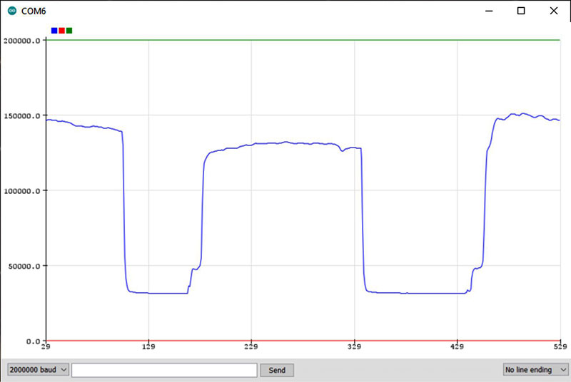
FIGURE 9. An example of the measured resistance in dim ambient light and with my finger over the sensor.
In the dim ambient light, the PSR sensor resistance was about 30K ohms. When my finger covered the PSR, the resistance went up to 130K ohms. The PPG instrument shown in Figure 10 is ready for its first measurements.
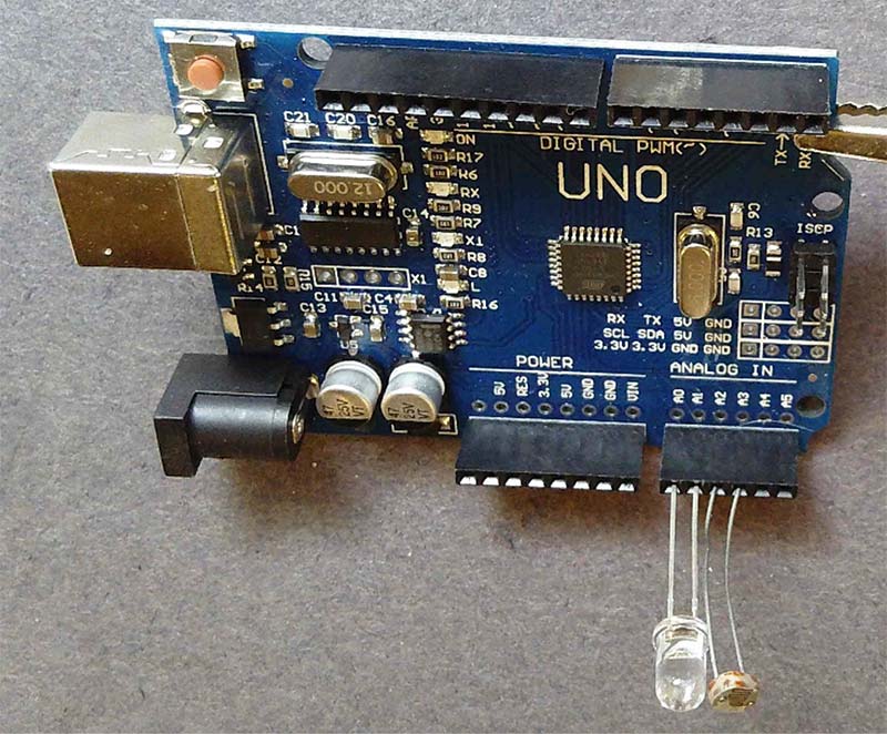
FIGURE 10. The PPG measurement system ready for the finger test.
Measure the PPG Effect in My Finger
With the LED on and the Arduino measuring and plotting the resistance of the PSR, all we have to do is place our finger over both the LED and the PSR, and watch the resistance change with our blood flow. I noticed the resistance was about 1.5K with my finger over the sensor, so I adjusted the scale to be 3K full scale. Figure 11 shows the first measured value of the PSR resistance.
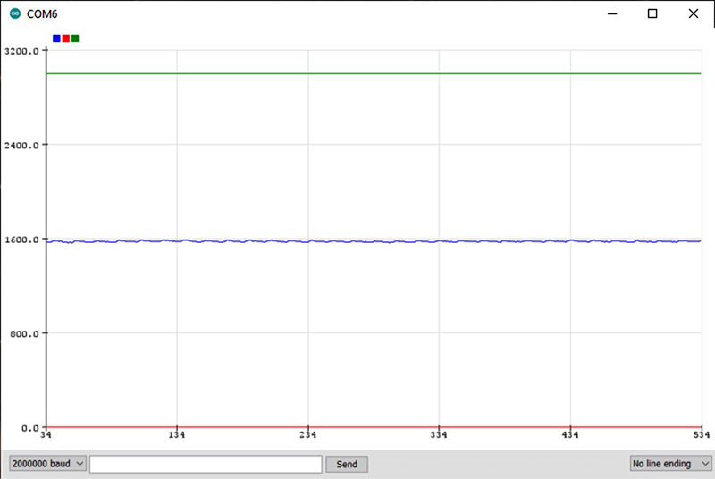
FIGURE 11. The first measured resistance of the PSR showing the very weak PPG effect.
This is the PPG effect. On this scale, it’s clear how small the effect is. It’s there, just very slight. If we auto scale it to show the small changes, the range of resistance changes is about 10 ohms peak-to-peak out of 1.6K, or less than 1%. Figure 12 shows this zoomed in scale.
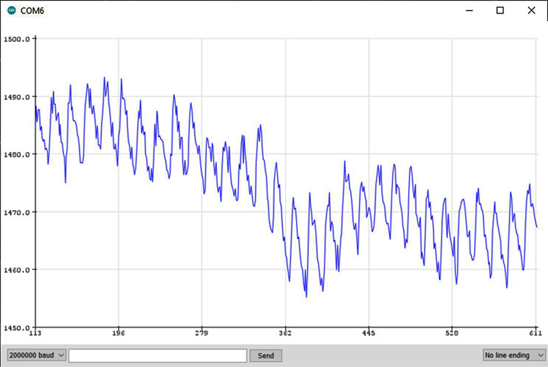
FIGURE 12. The PPG effect on a zoomed in, auto scaled plot.
If this is good enough for what you want to do, then you’re done. Have fun with your PPG instrument!
If you want to use this to modulate a light, for example, there is a small problem. The entire modulated signal is only 1% resistance change. As we move our finger around, this resistance level will change all over the place — much larger than the 1% modulation from our blood flow.
We would like to somehow compensate for the slower variations and subtract them off, so the PPG output signal is always centered about zero. This will make a much steadier PPG signal. This is where Trick #6 comes in.
Trick #6: Subtract a Running Average to Always Keep the PPG Signal Centered About 0
The last trick we’ll implement is to subtract off the running average so that slow fluctuations don’t affect the signal. A running average is not the same as the average of n points. What we really want to do is use a sliding window over the last n points, find their average, and display the current value with this average of the last n points subtracted off.
Then, for the next point, calculate a new average of the last n points and subtract it off. This way, we’re looking at each new measurement with the previous average subtracted off. The window over which we’re averaging runs along with the new data points as they come out.
There are a number of ways of implementing this running average. If the variations in the measurements we want to subtract off are random, there’s a simple method to use that doesn’t require storing an array of the last n points.
However, our measurements are not going to be random. They will slowly vary depending on the motion of our finger. An array which stores the last n points is the way to go. Here is the algorithm:
√ Select the number of points in the running average.
√ Initialize a buffer based on the first measured point.
√ Each time a new point is measured, add it to the end of the buffer.
√ Calculate the average of the buffer.
√ Subtract this average from the next new point that comes in.
√ Shift all the stored points up one in the array.
√ Repeat the process for each new point.
In the Arduino Uno with the ATmega 328 microcontroller, there is not much memory. This means the largest array of floating-point numbers we can use is about 300 before we get an out of memory error. If we average each point over three power line cycles or 50 msec, 300 points would give us a moving average window of 15 seconds. We can experiment with 1 to 300 points to find the optimum value.
The complete sketch which implements the running average is:
float V_meas;
float V_internal = 4.99;
float R_pin = 38000.0;
float R_PSR;
long iTime_ave_usec = 3.0 / 60 * 1e6;
long iCounter;
long iTime0_usec;
const int npts_RunningAve = 50;
float R_RunningAve;
float R_array[npts_RunningAve + 1];
float R_value;
void setup() {
pinMode(A0, OUTPUT);
pinMode(A1, OUTPUT);
pinMode(A2, INPUT_PULLUP);
pinMode(A3, OUTPUT);
digitalWrite(A0, HIGH);
digitalWrite(A1, LOW);
digitalWrite(A3, LOW);
Serial.begin(2000000);
//initialize the buffer:
for (int i = 1; i <= 1000; i++) {
V_meas = analogRead(A2) / 1023.0 * 5.0;
}
R_PSR = R_pin * V_meas / (V_internal - V_meas);
for (int i = 1; i <= npts_RunningAve; i++) {
R_array[i] = R_PSR;
}
}
void loop() {
V_meas = 0.0;
iCounter = 0;
iTime0_usec = micros();
while ((micros() - iTime0_usec) < iTime_ave_usec) {
V_meas = analogRead(A2) / 1023.0 * 5.0 + V_meas;
iCounter++;
}
V_meas = V_meas / iCounter;
R_PSR = R_pin * V_meas / (V_internal - V_meas);
//shift the array
for (int i = 1; i <= (npts_RunningAve - 1); i++) {
R_array[i] = R_array[i + 1];
}
R_array[npts_RunningAve] = R_PSR;
//calc average
R_RunningAve = 0.0;
for (int i = 1; i <= (npts_RunningAve); i++) {
R_RunningAve = R_array[i] + R_RunningAve;
}
R_RunningAve = R_RunningAve / npts_RunningAve;
R_value = R_PSR - R_RunningAve;
//Serial.print(R_PSR, 3); Serial.print(“, “);
//Serial.println(R_RunningAve);
Serial.print(-100); Serial.print(“,”);
Serial.print(100); Serial.print(“,”);
Serial.println(R_value);
}
I found a convenient number of running average points is 50. This is an average of about 2.5 seconds. To test the running average, I plotted the value of the PSR resistance for each point and the running average value. They match exactly as expected, shown in Figure 13.
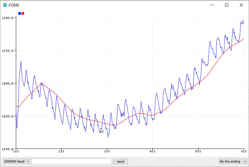
FIGURE 13. An example of the PPG signal and its running average.
When the running average is subtracted from each individual PSR resistance measurement, the range was within ±100 ohm. I set the scales to be this range. With a little trial and error, you can find the best scales for your PPG signal.
When this code runs and I place my finger over the LED and sensor, the scaled values of my PPG signal with the running average subtracted off is shown in Figure 14.
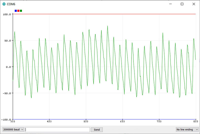
FIGURE 14. The scaled PPG signal with the running average subtracted off.
Conclusion
We are done. To see your PPG signature, grab your Arduino. Insert the LED into A0 and A1. Insert the photo-sensitive resistor into A2 and A3. Copy and paste this sketch into your Arduino from the article downloads, upload, and then open up your serial plotter tool. You too can observe the blood pulsing through your finger.
Start to finish is less than 10 minutes. If you already have the ultra-bright LED, Arduino, and photo-sensitive resistor, it’s free. If you buy them all off the shelf from AliExpress, it’s about $6 for all three parts.
It doesn’t get any easier than this. NV
Links
100 Bright LEDs on Amazon: https://www.amazon.com/CHANZON-PC-59042-Emitting-Assorted-Arduino/dp/B01AUI4VSI/ref=pd_all_pref_2/147-7601643-9932921?_encoding=UTF8&pd_rd_i=B01AUI4VSI&pd_rd_r=9ecc34f9-2f31-4957-9a08-1d999e867579&pd_rd_w=GDULr&pd_rd_wg=9MEjB&pf_rd_p=e6474b7e-8fb6-4ee2-b5d6-a1da55185fe6&pf_rd_r=PQ9C27NVWB71SHEW68KZ&psc=1&refRID=PQ9C27NVWB71SHEW68KZ
100 Bright LEDS on AliExpress: https://www.aliexpress.com/item/1936218827.html?spm=a2g0o.productlist.0.0.6cc57834cvCuBI&algo_pvid=4543c1d9-46e0-481f-8ee6-a60af4b8d91b&algo_expid=4543c1d9-46e0-481f-8ee6-a60af4b8d91b-3&btsid=0bb0623016038408882122775e622a&ws_ab_test=searchweb0_0,searchweb201602_,searchweb201603_
Arduino Uno on SparkFun: https://www.sparkfun.com/
Arduino Uno on AliExpress: https://www.aliexpress.com/
Photo-sensitive Resistor on Amazon: https://www.amazon.com/ZYAMY-50pcs-Photoresistor-Sensitive-Resistor/dp/B07XDW83MP/ref=sr_1_2?dchild=1&keywords=photosensitive+resistor+5516&qid=1603901053&sr=8-2
Photo-sensitive Resistor on AliExpress: https://www.aliexpress.com/item/32883143573.html?spm=a2g0o.productlist.0.0.71817584Cl8Yit&algo_pvid=12a066d9-a1b8-4c80-9471-0fec501f103e&algo_expid=12a066d9-a1b8-4c80-9471-0fec501f103e-4&btsid=0b0a556c16039003463108211ede21&ws_ab_test=searchweb0_0,searchweb201602_,searchweb201603_
Eric Bogatin received his BS in Physics from MIT and PhD from the University of Arizona also in Physics. He currently is an adjunct professor at the University of Colorado, Boulder where he teaches graduate EE classes. He also teaches Arduino workshops at Tinkermill, the Longmont Hackerspace. He’s written 18 books, many of them about low cost electronics projects.
Downloads
What’s in the zip?
Code Snippets