After reading the NV article on Ohm’s law, I thought a follow-up article that goes a little deeper might be in order. Specifically, how Ohm’s Law together with a computer and a couple of tricks can be used to calculate the time dependence of much more complex circuits involving not just resistors, but capacitors, inductors, op-amps ... you name it! Let’s skip the academic approach that you learned in EE101. Real world problems are usually too difficult for analytics. In this article, I’ll describe a simple numerical method that is intuitive and solves many complex problems with just a few lines of code.
Before diving into this, we need one more famous law: Kirchoff’s Law, which says that the sum of the voltages around a loop is always zero. Take a look at Figure 1 which is a circuit with two voltage sources and a capacitor. We want to know the voltage on the capacitor.
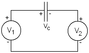
FIGURE 1. A simple circuit to illustrate Kirchoff’s Law.
Applying Kirchoff’s Law, we can write the loop equation:
V1 – VC – V2 = 0
It’s important to keep track of the polarities. Since the polarity of VC and V2 oppose the polarity of V1, those terms have a minus sign. Solving for VC, we have:
VC = V1 – V2
For our first problem, let’s find the time dependence of the voltage VC in the simple RC circuit of Figure 2.
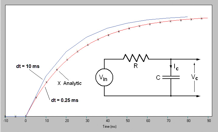
FIGURE 2. The simulated step response of an RC circuit with time constant RC = 25 ms. The X points are the analytical solution from Equation 1. The red curve is the numerical solution with dt = 0.25 ms. The blue curve is the numerical solution with dt = 10 ms.
Suppose that the input to the circuit is a step function; that is, the input voltage instantaneously goes from Vin = 0 to 10V at time t = 0. What is the time dependence of the output voltage? The analytic result using calculus is:
Vout(t) = Vin(1 – e-t/RC) Equation 1
Now suppose that the input is a square wave. For an analytic solution, we have to solve the circuit at every transition of the square wave until after a few cycles it settles down to a periodic waveform — a daunting task.
There’s a much easier way. Let’s use a computer and a little trick to get the complete solution in just a few lines of code. Here’s the trick: A capacitor can be described by the equation:
∆Vc = Ic ∆t / C Equation 2
This says that the change in the capacitor voltage ∆Vc in a short time ∆t is equal to Ic ∆t / C, where IC is the current flowing into the capacitor. For very short times, the change in voltage is very small so we can approximate the capacitor as a voltage source with a voltage VC. This makes the calculation of IC very simple. Using both Ohm’s Law and Kirchoff’s Law, we can write:
Vin – ICR – VC = 0
Solving for IC:
IC = (Vin – VC) / R Equation 3
With IC known, we can calculate a new VC (∆t) from Equation 2 and then a new IC and VC (2∆t) from Equations 2-3, and continue in a loop to obtain the complete time dependence VC(t) This is called the numerical method.
Let’s first do the step function problem so we can check the result against Equation 1. Code Example 1 is the simple basic code to simulate the voltage across the capacitor of Figure 2 in response to a step voltage input.
R = 5.0 ‘5 kohm
C = 5.0 ‘5 microfarad, RC = 25 ms
VC = 0 ‘Starting capacitor voltage (volts)
t = -10 ‘Start time (ms)
dt = 0.25 ‘Time increment (ms)
WHILE t< 90 ‘Compute for t = -10 to +90 ms
Input1: IF t>= 0 THEN Vin = 10 ELSE Vin = 0 ‘Create a 10V step at t = 0
IC = (Vin - VC) / R ‘Current into the capacitor (Ohm’s Law)
VC = VC + IC * dt / C ‘Update capacitor voltage
t = t + dT ‘Increment the time
Plot (t, VC) ‘A plotting subroutine defined elsewhere
WEND
END
CODE EXAMPLE 1. RC circuit step response simulation.
The critical code lines that simulate the circuit behavior are shown in red. Just to be clear, throughout this article I’m using the self-consistent set of units shown in Table 1.
| Parameter |
Unit |
Symbol |
| Voltage |
volts |
V |
| Current |
milliamperes |
mA |
| Resistance |
kohms |
k |
| Capacitance |
microfarads |
μF |
| Inductance |
Henrys |
H |
| Time |
milliseconds |
ms |
| Frequency |
kiloHertz |
kHz |
TABLE 1.
The results of the simulation are shown in Figure 2 which also shows that when we choose the time increment dt = 0.25 ms (100 times less than R x C), the numerical solution (red curve) is in perfect agreement with the analytic result (x points). With dt only 2.5 times less than RC (blue curve), the error is significant.
With dt ≈ RC/100 = 0.25 ms, the calculation takes 360 time increments which (on my computer) completes in less than one second.
Now, let’s change the input to an offset square wave and make the circuit a bit faster by setting C = 10 μF and R = 1 kΩ (RC = 10 ms). Implementing a 0.2 kHz square wave can be done by changing the line labeled “Input1” as follows:
Input1: If t >= 0 THEN Vin = 5 + 4 * SGN(SIN(2 * Pi * 0.2 * t) ELSE Vin = 0
The SGN function returns +1 for a positive argument and -1 for a negative argument, and therefore converts the sine wave to a square wave. Refer to Figure 3.
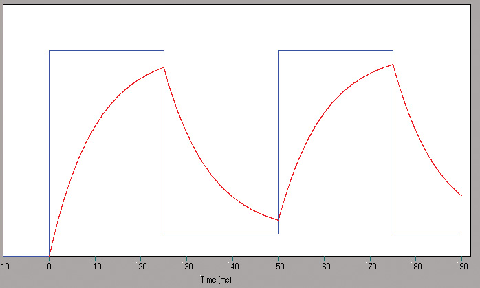
FIGURE 3. The output (red curve) of the circuit in Figure 1 with a square wave (blue curve) input.
Now, let’s add an inductor as shown in Figure 4.
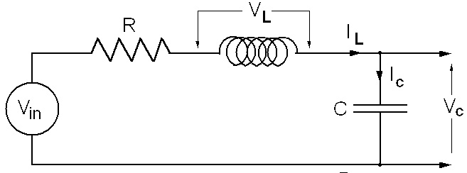
FIGURE 4. An RLC circuit.
The equation describing an inductor is identical to Equation 2 but with C replaced by L and current and voltage reversed; that is, the change in the current through an inductor ∆IL in a short time ∆t is equal to where VL∆t / L is the voltage across the inductor:
∆IL= VL∆t / L Equation 4
By the same logic, for short times an inductor can be treated as a constant current source. In order to update the capacitor voltage and inductor current at each time increment, we need equations for IC and VL.
The code to simulate this circuit is basically the same as Code Example 1 but with the red highlighted lines of Code Example 1 replaced by Code Example 2.
IC = IL ‘Current into the capacitor
VL = Vin – IL * R - VC ‘Voltage across the inductor
VC = VC + IC * dt / C ‘Update capacitor voltage
IL = IL + VL * dt / L ‘Update inductor current
CODE EXAMPLE 2. Step response of an RLC circuit.
The result of the RLC simulation is shown in Figure 5. Now, it’s time to apply these ideas to a practical problem.
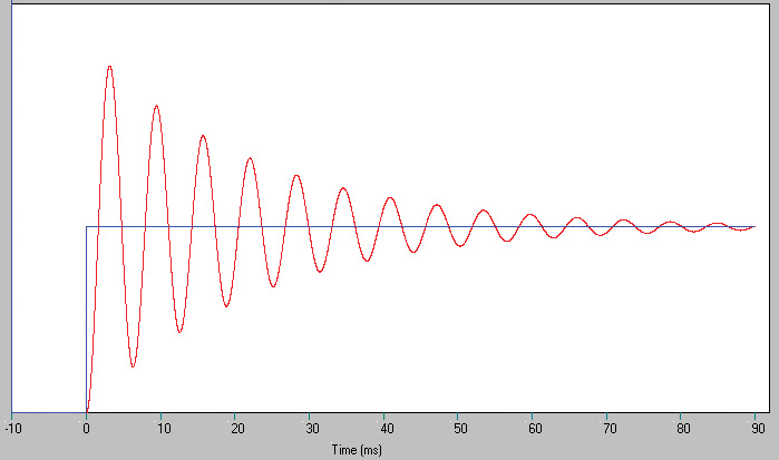
FIGURE 5. The computed step response Vc of the RLC circuit in Figure 4. Component values are R = 0.1 kohm, C = 10 μF, and L = 0.1 H.
Let’s look at another article in the May-June 2018 issue on sine wave generators. Specifically, the circuit in Figure 4 on page 86 (Open Communication column); shown here as Figure A.
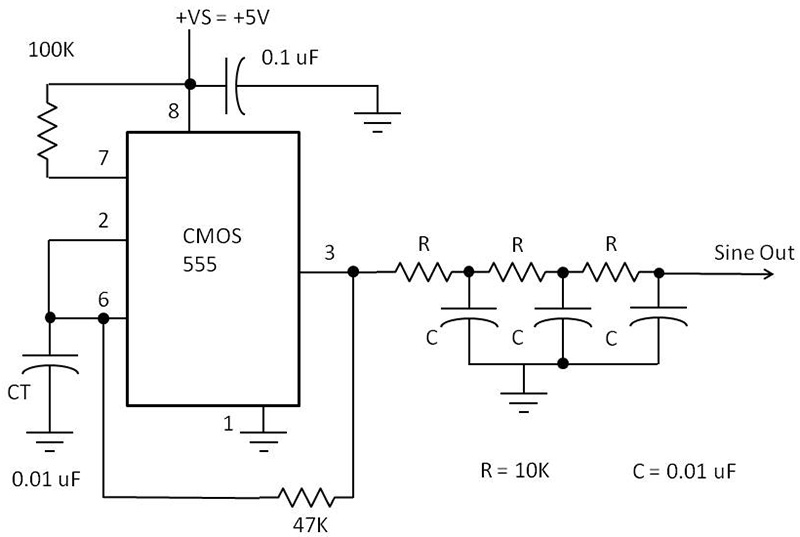
FIGURE A. Circuit from the Open Communication column.
This circuit creates a sine wave by filtering out the fundamental of a square wave using a three-stage RC filter. I have drawn the filter part of this circuit in Figure 6.
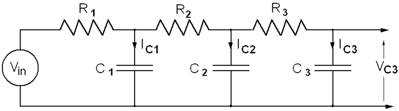
FIGURE 6. A three-stage RC filter.
The component values for this example are R1 = R2 = R3 = 5 kohms and C1 = C2 = C3 = 0.1 μF. The square wave input frequency is f = 0.5 kHz. In this circuit, C1 and C2 receive current from both sides so the equations for the current into these capacitors have two components as shown in the first two lines of Code Example 3.
IC1 = (Vin – VC1) / R1 + (VC2 – VC1) / R2
IC2 = (VC1 – VC2) / R2 + (VC3 – VC2) / R3
IC3 = (VC2 – VC3) / R3
VC1=VC1 + IC1 * dt / C1
VC2=VC2 + IC2 * dt / C2
VC3=VC3 + IC3 * dt / C3
CODE EXAMPLE 3. Simulation of a three-stage filter.
The complete simulation code is obtained by replacing the highlighted lines of Code Example 1 with Code Example 3 and (of course) assigning the values of C1-3 and R1-3.
Figure 7 shows the computed time-dependent voltage across each capacitor. The simulation clarifies the trade-off in this design. Each of the three stages improves the approximation to a sine wave at the expense of decreased amplitude.
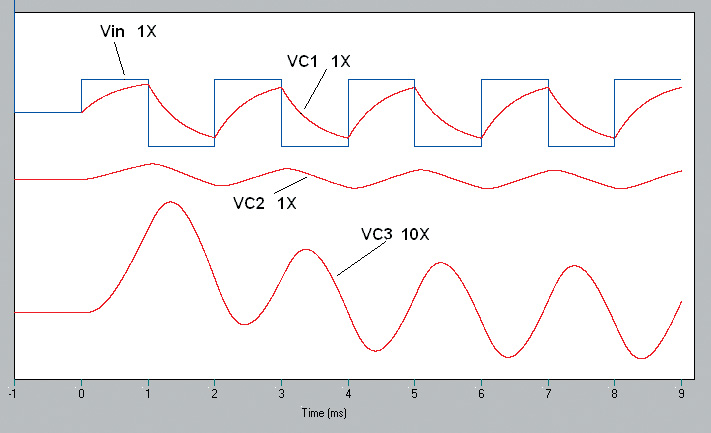
FIGURE 7. Simulation of a filter to convert a square wave to a sine wave.
A larger value of RC will make a better sine wave, but with a smaller amplitude. For this simulation, I chose RC = 0.25/ f = 0.25/0.5 = 0.5 ms. (The May-June article chose RC = 0.16 / f which generates more like a slightly rounded triangle wave.)
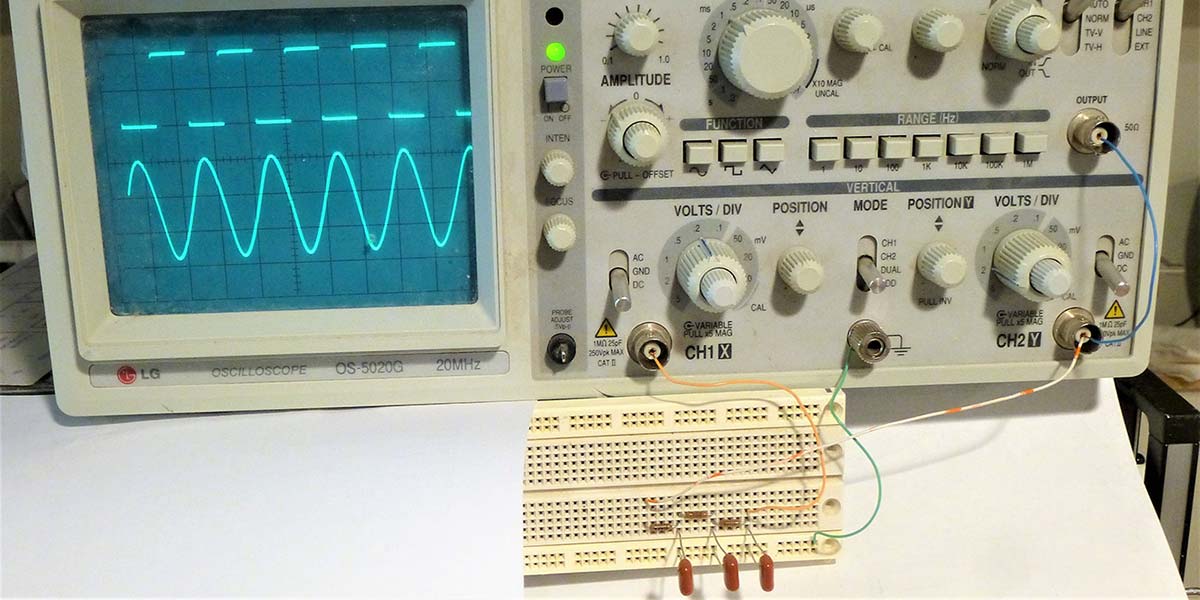
In Figure 8, I have breadboarded the circuit of Figure 6. My oscilloscope happens to include a function generator, so I can create and view both the input (top trace, 1V/div) and output (bottom trace, 0.1V/div) with just my oscilloscope.
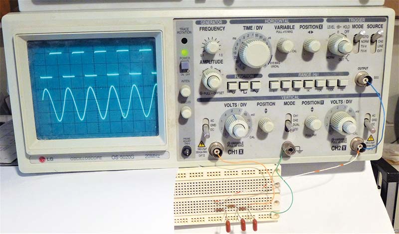
FIGURE 8. A breadboard test showing the input and output of the three-stage filter circuit in Figure 6. Note that the top trace is at 2V/div and the bottom trace is at 0.2V/div as in the Figure 7 simulation.
There are plenty of circuit simulation programs that will easily solve the problems I’ve discussed so far, but when the problem also includes mechanical components those canned simulators probably won’t work. Stabilizing the inverted pendulum is a nice hybrid problem involving both electronic and mechanical components. (See my article on this topic in the December 2017 issue of SERVO Magazine; www.servomagazine.com.)
The simulation of this problem involves both electrical and mechanical components involving a motor, gravity, mass, inertia, velocity, positions, and angles. Figure 9 is a diagram of an inverted pendulum stabilization system with just the basics needed to write a simulation code.
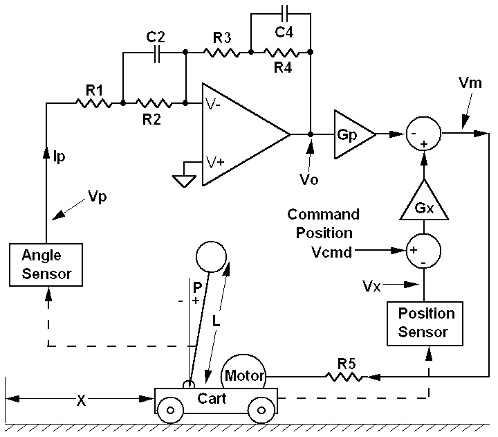
FIGURE 9. The control system to stabilize an inverted pendulum and track a command position.
The inverted pendulum is attached to a motor-driven cart by a free pivot. Sensors measure the cart position and the pendulum angle from vertical. These two signals feed into the control system to produce an output signal that drives the motor. The system must keep the pendulum upright and simultaneously track a command position input. If you’re wondering about the design details, refer to my article. Our job here is to simulate the existing design in Figure 9. Writing the equations for this system is a bit more complicated. First, let’s address the operational amplifier. An op-amp simply takes the voltage difference between its two inputs and multiplies it by a large gain factor, typically on the order of 100,000. When there is feedback as in Figure 9, the gain is reduced and given by the ratio of the feedback impedance (R3, R4, C4) to the input impedance (R1, R2, C2). Capacitors C2 and C4 make it possible to shape the frequency response.
To write the simulation equations, we just need to know two things: (1) When the op-amp positive input is grounded as in Figure 9, the high gain and feedback cause the negative input to become a virtual ground; that is, the voltage at the negative input will be essentially zero. (2) No current flows into the op-amp input terminals, which in the case of Figure 9 means that the current flowing to the right in R3 equals the current flowing to the right in R1.
Now, we can write the simulation equations starting with the current Ip. Since V- = 0, the equation is:
Ip = (Vp – VC2) / R1
Vp is the voltage output of the angle sensor when the pendulum is leaning at an angle of P degrees. This is the first line in the simulation code listed in Code Example 4.
1: Ip = (Vp - VC2) / R1 ‘The input current through R1
2: IC2 = Ip - (VC2 / R2) ‘The current into C2
3: IC4 = Ip - (VC4 / R4) ‘The current into C4
4: Vo = -(Ip * R3 + V4) ‘Filter output (inverted)
‘Xdd is the acceleration to be applied to the cart for time dt
6: Xdd = -Gp * Vo + Gx * (Vcmd -Vx) ‘Close the angle and position loops
‘Compute the rotational acceleration of the pendulum
8: Pdd = (1 / L) * (g * Sin(P) - Xdd * Cos(P) - Xd * Pd * Sin(P))
9: V2 = V2 + I2 * dt / C2 ‘Update capacitor voltages V2 and V4
10: V4 = V4 + I4 * dt / C4
11: Xd= Xd+ Xdd *t ‘Update the cart speed
12: X = X + Xd* dt ‘Update the cart position
13: Pd = Pd + Pdd * dt ‘Update the pendulum rotation rate
14: P = P + Pd* dt ‘Update the pendulum angle
15: t = t + dt ‘Update the time
16: DrawCP ‘Draw the cart and pendulum to the screen
17: Goto 1
CODE EXAMPLE 4. Simulation of an inverted pendulum on a motor-driven cart.
Code lines 2-3 find the current into capacitors C2 and C4. Line 4 follows from the fact that V- = 0. Line 6 sums up the signals that drive the motor, including gain factors Gx and Gp that scale the cart acceleration Xdd to Vm — the voltage applied to the motor through R5.
Code line 8 shows how the acceleration Pdd of the pendulum tilt angle P depends on its length L, the acceleration of gravity g, the tilt angle P, the cart acceleration Xdd, the cart velocity Xd, and the rate of change Pd of the pendulum tilt angle. The derivation of this equation is beyond the scope of this article, but more info can be found on Wikipedia; look up “Inverted Pendulum.”
We now have everything needed to update the state of the system. Lines 9-10 update the capacitor voltages. Line 11 updates the cart speed Xd based on the known acceleration Xdd and then line 12 updates the cart position X based on the known speed Xd. Lines 13-14 perform the same operations to update cart tilt angle P, then update the time and the animation, and then go back to line 1 to compute the next time increment. Refer to Figure 10.
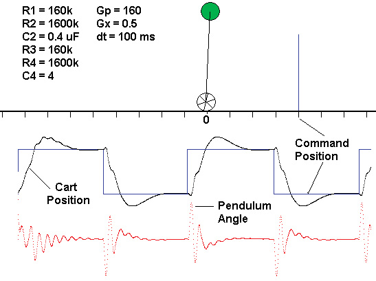
FIGURE 10. Simulation results for the inverted pendulum. The top drawing is the animation at time = 0, scaled at one meter per division. The vertical blue line shows the command position at time = 0, and the blue square wave below shows how the command position changes with time (oscillating from -5m to +5m every 30s). The black curve is the cart position and the red curve is the pendulum angle (max deviation from vertical is about ± 10 deg), all as a function of time.
Of course, if you have a circuit simulator on your computer you can get the results of Figures 2, 3, 5, and 7 without writing any code.
Aside from not needing a simulator, the beauty of the numerical method described in this article is the insight it gives to circuit operation and the easy adaptability to problems involving more than just electronic components; for example, the dynamic behavior of the mechanical parts in the inverted pendulum problem.
Springs are like inductors, mass is like capacitance, Ohm’s Law becomes Newton’s F = MA. You could analyze a bridge truss by noting that the beams are like very stiff springs. NASA could never navigate a spacecraft to Pluto without the numerical method. NV