A flashback to the ‘80s ...
The Teensy 4.0 and 4.1 microcontrollers from pjrc.com are a game changer. They are a quantum leap in CPU speed and processing power. Here are the specifications:
- ARM Cortex-M7 at 600 MHz
- Floating Point Math Unit; 64 and 32 bits
- 1984K Flash, 1024K RAM (512K tightly coupled), 1K EEPROM (emulated)
- USB Device 480 Mbit/sec and USB Host 480 Mbit/sec
- 40 Digital Input/Output Pins, 31 PWM Output Pins
- Seven Serial, three SPI, three I2C Ports
- Two I2S/TDM and one S/PDIF Digital Audio Port
- 14 Analog Input Pinsexercising-the-teensy-4.0
- Three CAN Busses (one with CAN FD)
- 32 General-Purpose DMA Channels
- Cryptographic Acceleration & Random Number Generator
- RTC for Date/Time
- Programmable FlexIO
- Pixel Processing Pipeline
- Peripheral Cross Triggering
- Power On/Off Management
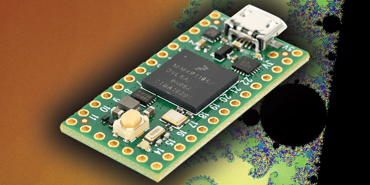
The numbers that caught my attention were 600 MHz (actually it can be overclocked up to 1.008 GHz, with cooling) and 64-bit floating point math.
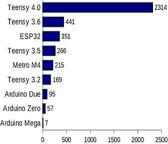
Figure 1. CoreMark benchmarks of various microcontrollers.

Figure 2. Teensy 4.0 pin layout and functions card, front side.
Figure 3. Teensy 4.0 pin layout and functions card, back side.
My first thought was what kind of program could use this level of performance and Mandelbrot images came to mind — a favorite programming pastime of mine.
The Mandelbrot Math
The Mandelbrot set is computed by operating on a fairly simple equation that contains complex numbers of the form:
x + yi where i = sqrt(-1)
The Mandelbrot equation is:
zn+1 ← zn² + c
where
z = x + yi and c = a + bi
substituting these values into z² + c, we have:
(x + yi)² + a + bi
x² + 2xyi - y² + a + bi
separating the real and imaginary parts of z gives:
x ← x² - y² + a
y ← 2xy + b
To determine whether a point (a,b) in the complex plane is a member of the Mandelbrot set, the real and imaginary parts of the equation are iterated. The x and y values are first initialized to zero. The constants a and b — the point in the plane (which becomes a point on the computer screen) — are then substituted into the equations giving
x ← a and y ← b
for the first iteration.
The two new values for x and y (along with the constants a and b) are now substituted into the equations again. This looping procedure (iteration) continues until the absolute value of x + yi > 2, i.e., sqrt(x² + y²) > 2.
For those cases where this value never exceeds two, the maximum number of iterations is preset. Otherwise, we’ll have an infinite loop in our program. A value of about 1000 is usually quite adequate, although this value is raised to several thousand when smaller details at high magnification are examined.
The number of times the equations are iterated before the value of sqrt(x² + y²) > 2 is called the dwell. I like to use a maximum dwell value of 1023, as it nicely fits a color palette length of 1024. Notice that zero is a valid dwell value, so dwells of the range 0 to 1023 constitute 1024 different values.
Those initial points (a,b) (where the dwell is infinite or for more practical purposes attains the preset maximum) are members of the Mandelbrot set. Another way to describe this is to say that for points within the Mandelbrot set, the sequence of points produced by this iteration procedure is bounded inside a circle of radius 2, where points outside the set are unbounded and continue to grow and escape the circle. The sqrt(x² + y²) for points in the Mandelbrot set never grows larger than two no matter how many times we iterate the calculations.
The Mandelbrot set exists entirely within the area defined by:
-2 <= a <= 2 and -2 <= b <= 2
in the complex plane. A Mandelbrot image is produced by taking this area of the complex plane and dividing it into an array of say 1200x1200 points. Each one of these points becomes the constant (a,b). The iteration procedure previously described is used on each of the 1.44 million points, coloring each point in the Mandelbrot set black and all others white. The algorithm is:
// Generate Mandelbrot Set in Black and White
maxcount = 1023 // 1023 for palette fit
for b = 2 to -2 stepdown 1/300 // 1200 points in y
for a = -2 to 2 step 1/300 // 1200 points in x
x = 0 // initialize everything
y = 0 // to zero and start the
count = 0 // iteration loop
while (sqrt(x*x + y*y) < 2) and (count < maxcount)
x = x*x – y*y + a // real part of equation
y = 2*x*y + b // imaginary part
count = count + 1 // add 1 to loop count
end while
if count = maxcount plot(a,b,BLACK) // when loop ends
else plot(a,b,WHITE) // did the count
end for a // end up at our
end for b // maximum, if so
// it’s in the
// Mandelbrot set
While the algorithm is not that complex, the amount of computation is enormous. Depending on the programming language and style, the inner loop has at least four multiplications and a square root. For a point in the Mandelbrot set, this loop is executed 1023 times and there are over a million points to check! It’s not surprising that the Mandelbrot set was not discovered until the age of computers.
In the Mandelbrot program, some additional refinements are made to standardize the initial parameters used to generate a specific image.
Instead of defining the range of (a,b) values used for an area, a center point and a magnification are specified.
We do this because almost all the Mandelbrot images we wish to produce are magnifications of a tiny area.
A magnification value is easier to specify than defining a tiny area such as -.077 to -.07701 in the x direction and 0.170 to 0.17001 in the y direction. The center point is simply a chosen (a,b) value. The length of a side of a square which encloses the area of interest is defined as
side = 2/magnification
such that a magnification of one would give us an area of one unit on a side.
Therefore
magnification = 2/side
and the following values can now be defined as:
a_minimum = a_center - side/2
the smallest x value in the enclosed square and
b_maximum = b_center + side/2
the largest y value in the enclosed square.
In addition:
gap = side/width
where width is defined as the number of points that make up a side (or on a computer screen the number of pixels) and the gap being the distance in the plane between each point.
The values defined above are shown in an example in Figure 4.
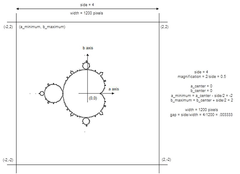
Figure 4. The parameter definitions.
There are a couple of standard programming tricks we use to make the computation more efficient. First, we don’t really check to see if the sqrt(x² + y²) > 2. Instead, we check to see if (x² + y²) > 4, eliminating a square root we won’t have to calculate. Second, looking at the equation:
y = 2*x*y + b
it makes more sense to write this as
y = (x+x)*y + b
This saves us a multiplication which is significant when the inner loop consists of six multiplications and is now reduced to five. By including the squaring of x and y in our (x² + y²) > 4 test, we can further reduce the multiplications to three.
The Mandelbrot set shown in Figure 5 is an interesting image; a sort of cardioid with a spiked head attached at the left.
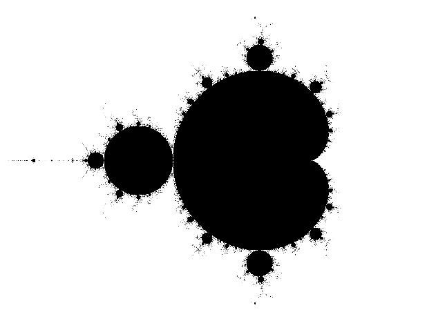
Figure 5. The Mandelbrot set.
The boundary of the set sprouts self-similar buds of different sizes. Vastly more interesting images are forthcoming when we examine the boundary areas of the Mandelbrot set under higher magnification.
To obtain higher magnifications, we can simply divide a smaller area into our array of points. For example, the area defined by the center point (-0.77,0.17) and magnification 20 is located in the upper valley between the head and the cardioid shaped body. This area has been named Seahorse Valley and is illustrated in Figure 6.

Figure 6. Magnification of 20 at center point (-0.77, 0.17).
If we continue with these magnifications, very different and interesting images can be produced by coloring the dwell values in specific ways. Along with coloring points in the Mandelbrot set black, we can assign different colors to other points based on their dwell value. For example, we might assign yellow to dwell values in the range 10 to 19, red to 20 to 29, etc.
When we do this, a great deal more detail begins to appear in the boundary regions. This region of interest exists only in a narrow band just outside and at the edge of the Mandelbrot set.
The program developed here uses a 1024 color palette to color the dwell values. Figure 7 shows the same area as Figure 6 but uses a color palette to represent the different dwell values.
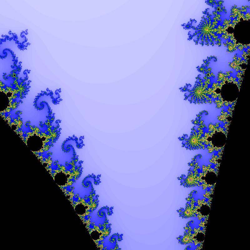
Figure 7. Magnification of 20 at center point (-0.77, 0.17) with coloring.
A dwell value of 10 is assigned color index 10 in the 1024 color palette, dwell 11 is assigned index 11, etc. Dwell values over 1023 (there is a dwell value of 0) are assigned a value of modulo(dwell/1024).
The color palettes contain smooth transitions of one color to another, creating very attractive images. Later, as we develop the program, we’ll use a few other programming tricks to manipulate the palette to act like one of different lengths from 32 to 4096.
Images that contain mostly low dwell values look better colored with smaller palettes, and ranges of higher dwell values look better with palettes of greater length.
The Test Circuit
A seven inch Nextion display was chosen to display the Mandelbrot images because I wanted the simplest circuit possible to test the Teensy 4.0. The Nextion display, Teensy 4.0, and a small five volt fan for cooling are the entire circuit.
When overclocking at 912 MHz or higher, the fan is required. Figure 8 shows the test circuit.
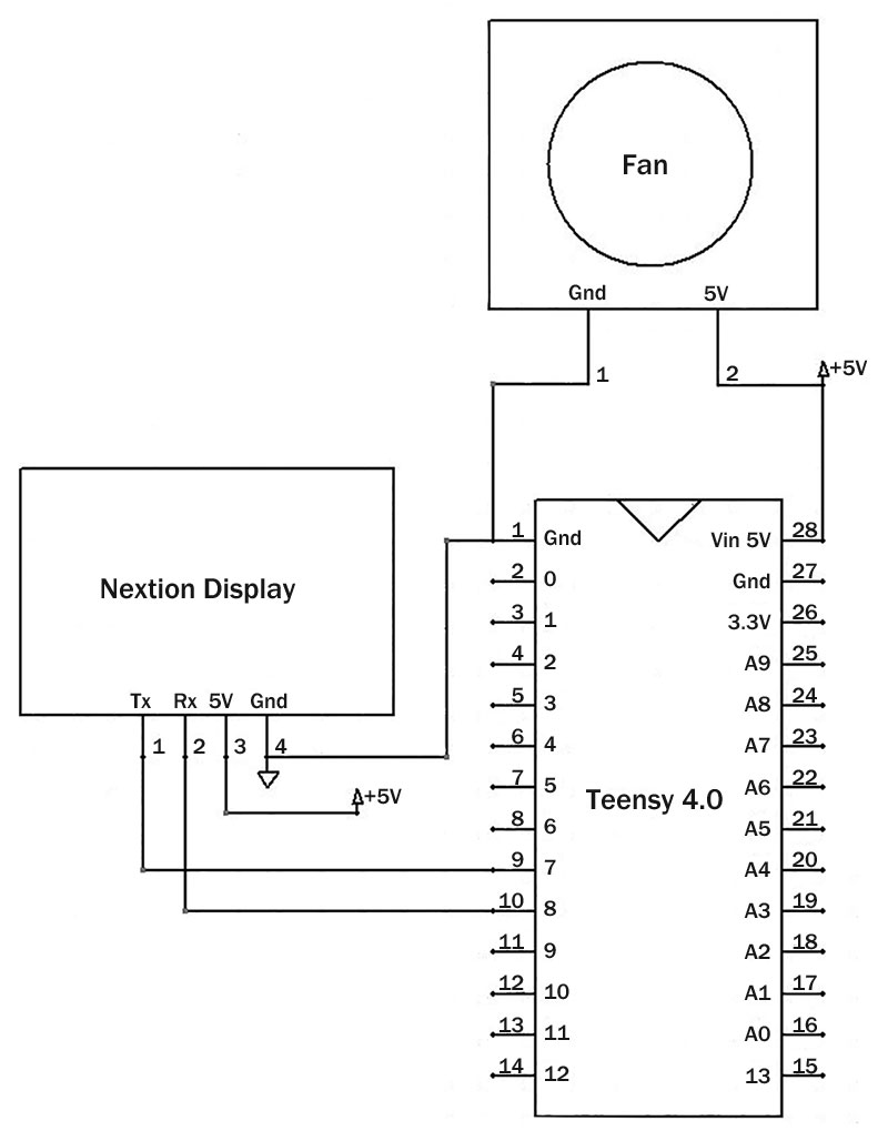
Figure 8. The test circuit.
Figure 9 shows the circuit on a breadboard.
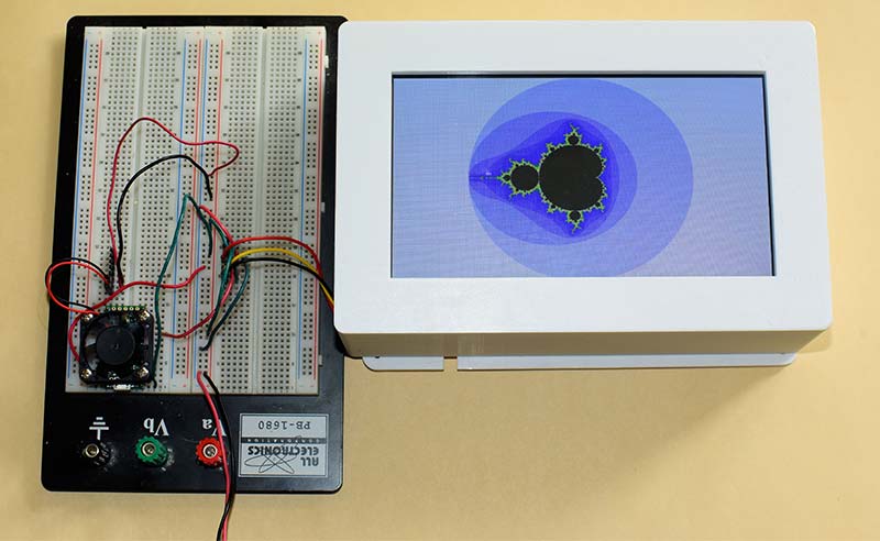
Figure 9. The circuit on a breadboard; the Teensy 4.0 is under the small fan.
Figure 10 is one of the Mandel images I created.
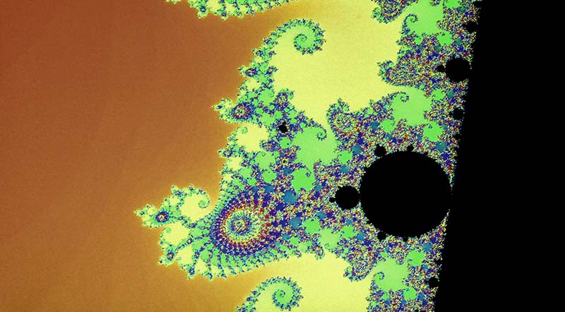
Figure 10. The Nextion display can produce some impressive images.
The Program
For programming, the Arduino IDE (integrated development environment) was used. The seven inch Nextion display has a resolution of 800x480 pixels. Because the display is not a square, some programming changes were necessary. The Nextion also uses 16-bit color and this needs to be accommodated as well.
As the Mandel_Machine program is described next, there are a few other tricks that will be revealed. The program can be found in the downloads.
The mandel() function in the program does the majority of the computing. There are only three other functions: genPalSegmentnew() to generate different palettes; drawPallete() to draw the palette on the Nextion display; and writeString() to write commands to the Nextion display.
The mandel() function begins by creating one of the three palettes described in the palette[3][24] array. The first two are color and the last is grayscale. There’s a lot of bit manipulation here and then each color is shifted into a 16-bit unsigned integer.
Next, the color palette is drawn on the Nextion display and the variables are set to their initial values. The main loop then computes the dwell value for each pixel in the image.
Because a line can have several pixels of the same color, we wait until the color changes in a line and then draw a line to the screen. This reduces the number of writes to the Nextion display.
My first attempts at using this program were with a 3.5 inch Nextion display which contains a 48 MHz MCU. The 3.5 inch Nextion could not keep up with the Teensy 4.0.
It would get buffer overflow on the serial port — even running at 921600 baud — which then shows up as drawing errors. I inserted delays in the program to get things to work. This problem went away with the seven inch Intelligent Nextion display which has a 200 MHz MCU.
After recording the times to generate each image, it became obvious that even with the faster seven inch Nextion display, the overall time was mostly dependent on the Nextion’s speed. Increasing the speed from 600 MHz to 1008 MHz on the Teensy 4.0 did not reduce the overall time on many images by much.
On images where the total number of iterations was substantially higher, the time to generate an image was significantly reduced with increased clock speed. By increasing the maximum dwell value from 5,000 to 65,000, this reduction is more apparent.
At this point, the increased computation needed with 65,000 for the maximum dwell demonstrated the Teensy 4.0’s power when the CPU was overclocked. Refer to Table 1.
| Image Number |
Maxdwell = 5,000 CPU Speed = 600 MHz Seconds |
Maxdwell = 5,000 CPU Speed = 1008 MHz Seconds |
Maxdwell = 65,000 CPU Speed = 600 MHz Seconds |
Maxdwell = 65,000 CPU Speed = 1008 MHz Seconds |
Billions of Iterations with Maxdwell = 65,000 |
| 0 |
12.10 |
8.78 |
111.42 |
67.86 |
1.41 |
| 1 |
22.48 |
18.38 |
145.21 |
91.37 |
1.76 |
| 2 |
22.30 |
18.24 |
143.11 |
90.11 |
1.72 |
| 3 |
79.17 |
75.73 |
81.86 |
77.34 |
0.49 |
| 4 |
59.85 |
58.96 |
61.25 |
59.79 |
0.18 |
| 5 |
76.83 |
75.77 |
99.55 |
89.29 |
0.53 |
| 6 |
68.34 |
53.88 |
495.95 |
308.29 |
1.72 |
| 7 |
25.20 |
23.42 |
25.20 |
23.42 |
0.09 |
| 8 |
67.65 |
67.31 |
67.65 |
67.31 |
0.13 |
| 9 |
49.54 |
48.53 |
49.54 |
48.53 |
0.12 |
| 10 |
100.33 |
99.81 |
100.36 |
99.83 |
0.47 |
| 11 |
91.86 |
91.38 |
91.87 |
91.39 |
0.34 |
| 12 |
54.81 |
54.34 |
54.81 |
54.34 |
0.12 |
| 13 |
17.01 |
15.60 |
59.06 |
40.61 |
0.61 |
| 14 |
32.38 |
25.96 |
223.50 |
139.66 |
2.72 |
| 15 |
31.40 |
30.40 |
50.99 |
42.05 |
0.34 |
| 16 |
26.74 |
26.02 |
26.74 |
26.03 |
0.08 |
| 17 |
62.58 |
62.58 |
62.60 |
62.59 |
0.06 |
| 18 |
72.63 |
72.59 |
73.33 |
73.01 |
0.08 |
Table 1. Program speeds in seconds.
The Teensy 4.0 does have impressive computing power: over a billion iterations, each with three 64-bit multiplications, four additions, one subtraction, and loop overhead in under a minute.
While the focus here is on the computing power of the Teensy 4.0, there are many other features that make it an excellent choice for many applications. NV
Downloads
What’s In The Zip?
Code and HMI File