There are probably thousands of operational amplifiers (op-amps) available. But which one is the best for your particular application? A datasheet has lots of numbers and graphs, and then there are the many strange acronyms. This article will show you how to wade through the jargon and select the op-amp that best fits your needs.
There are some basic items that need mentioning before we start. The first is that we will only examine basic op-amps. We will not look directly at special types, like high frequency (10s to 100s of MHz), current-difference, or trans-conductance. However, once the basic op-amp is understood, it is a small step to the special types.
Another point is that you have to know what your circuit needs. This seems obvious but it is sometimes overlooked. Trying to use a five-volt op-amp in a 25 volt circuit generally guarantees poor performance. More subtly, using an op-amp that doesn’t have the proper frequency range or is too noisy is not a rare occurrence. You must fully understand your requirements to make a proper selection.
An ideal op-amp has no distortion, uses no meaningful power, has infinite amplification, generates no noise, has infinite input resistance (to present no load to the signal being amplified), has infinite frequency response, accepts signals of any voltage and, of course, is free. While modern devices can come close to some of these ideals — like input resistance and low power — no amplifier can achieve them all.
Figure 1 illustrates some of the typical imperfections found in op-amps.
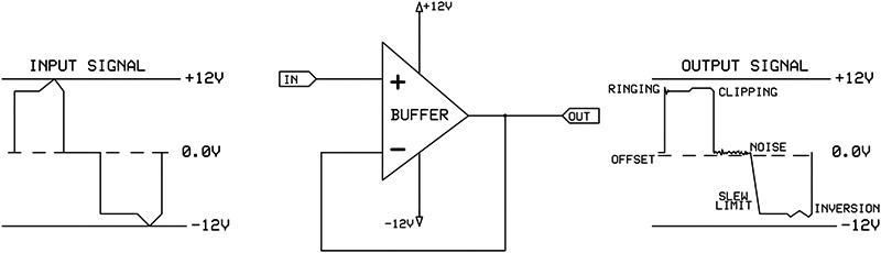
FIGURE 1. A real op-amp is not perfect. The output signal displays a number of typical failings. Note that the problems are only shown once for simplicity. Ringing occurs at every fast transition while noise is continuous, etc. You can imagine what the output signal looks like if all these errors were applied over the whole signal.
(Note that the problems are shown in isolation for clarity. In reality, most of these effects are continuous and compounded.) This means that you must choose between different amplifiers with different strengths and weaknesses. This is the typical situation of engineering trade-off.
Basic Op-Amp Specifications
All op-amp data sheets have a section labeled “Absolute Maximum Ratings.” I call these the “Fry Points” because operating the device at these (or higher) levels will fry it. You can never exceed these ratings and expect anything good to happen. You should always stay well below these values. The datasheet will usually specify, in some manner, standard maximum operating levels.
Many datasheets will have “Typical” numbers. A good engineer pretty much ignores them. The worst-case values should always be used to guarantee proper performance. If you are simply making one item for your own use, you might take a chance and/or hand-select an op-amp for your project. But this approach is not acceptable in a professional setting (except under rare and very special conditions).
The table of specifications in most datasheets is presented in alphabetical order. This may be useful in finding a specific value, but it does not provide any coherence to the information. Here, the specifications will be organized into groups that are related in some way. Four basic groups will be used: Power, Input, Output, and Frequency. Note that these groups are not independent of each other. Defining your design with these four factors is pretty straightforward and intuitive.
Power
First and foremost it must be noted that there is no “Ground” pin on an op-amp. Thus, any and all op-amps can operate from a single supply. So why are some op-amps specified as requiring positive and negative power supplies? This is because the input is assumed to be at ground and that AC input signals will move above and below ground. It is clear that if the input voltage exceeds either power supply (either more positive or more negative), bad things will happen. This is one of those notes mentioned in the Absolute Maximum Ratings entry. The input voltage MUST be within the range of the power supply. (More on this in the Input section.)
The operating voltage (identified as V+ and/or V-) is often specified in a separate table and/or in the text of the datasheet. Way back when, it used to be that ±15 volts (or even higher) was the standard (bipolar or dual power supplies). Nowadays, many op-amps are specified as needing between +3 to +15 volts (unipolar or single supply). This still means that the inputs to the op-amp must be within the power supply (although those noted as “single supply” op-amps allow the input to go to the negative rail ... usually ground).
Thus, negative voltages are not allowed at the inputs with this single supply specification. Also, the common use of two nine-volt batteries (one for V+ and one for V-) will result in 18 volts between the power terminals. This exceeds the Fry Point for these devices. So be careful to read the power specifications properly. Obviously, you know what voltages are available so this specification is easy.
The power supply rejection ratio (PSRR) identifies how sensitive the op-amp is to variations in the power supply. You don’t want power supply noise (from AC supplies) or drift (from batteries) to affect the output. This specification is listed as a decibel (dB) value where every increase by 20 dB is a 10-fold increase in the ratio. So, a 60 dB value here means that a one volt change in the power supply will cause a 0.001 volt (or one millivolt) change in the output.
This value depends on the actual power supply voltage, as well as the frequency of the noise. Higher operating voltages and lower noise frequencies generally result in better PSRR figures. Often, datasheets will provide graphs showing these variations.
Determining what you need for this parameter is not too difficult. If you are using an op-amp with digital logic (which typically causes a lot of power supply noise), you will want an op-amp with a good PSRR rating. If your op-amp is a fully analog design with a good, regulated analog power supply, then this parameter probably isn’t too important.
The current needed to power the amplifier is defined as the supply current (Is). This is the quiescent current. This does not include external components or any output current. If there are multiple amplifiers in a single package, this usually refers to a single amplifier. However, the datasheet will specify this. Clearly, battery-operated circuits will work longer with an amplifier that uses less power. Sometimes this is listed in milliwatts (or microwatts) as power consumption (Pd). So, you will have to convert it to mA (or µA) using the power supply voltages listed in the table.
Input
There are many input parameters and this group often contains the most important items that define the op-amp’s performance for a particular application.
The first basic specification is the input resistance (Rin) (sometimes it is referred to as input impedance). This indicates how much load the op-amp places on the signal. This value should be as high as possible (however, for very high speeds this will be relatively low because parasitic capacitance can affect the frequency response significantly). Obviously, you don’t want your op-amp to affect the signal you are amplifying. Values in the 100s of megohms are typical. Some of the newer op-amps have input resistances so high that they are not directly measurable ... greater that 10 teraohms! (A teraohm, or TΩ, is 1,000,000 megohms.) (Note that the input capacitance is not usually given, but is very low; on the order of a pF or so ... mostly due to the leads.)
Occasionally, older specsheets provide only an input bias current (Ib) rather than an actual input resistance. This says how much current is needed to drive the inputs. It can be roughly converted to an input resistance by using Ohm’s law with the supply voltage. For example: If the Ib is 170 nA (nanoamps) and the supply voltage is five volts, then Ohm’s law is 5V = 170 nA x Rin. Solving this gives about 29 megohms as the input resistance.
The input offset voltage (Vos) and input offset current (Ios) sound similar to the input bias current (above) but are very different animals. These refer to the inaccuracy of the amplifier and should be as close to zero as possible. If both inputs to the op-amp are zero, then the output should also be zero. But since the amplifier isn’t perfect, there will be some residual voltage at the output. So why not call this the output voltage error? This is because the gain of the circuit will affect the output. A circuit with a gain of 100 will increase this error by a factor of 100. That is why this is referred to the input rather than to the output. It appears to the circuit like a DC error at the input. In fact, the definition of offset error is the voltage (or current) applied to the input to force the output exactly to zero.
Offset errors are generally not too important to AC circuits because the effect is seen as a fixed DC error. Since AC circuits are generally capacitively-coupled, the DC problem goes away. However, large gains (1,000 or so) can turn a 5 mV Vos into a five volt DC error at the output. This could possibly cause the amplifier to try to generate an output voltage greater than the supply voltage and lead to clipping.
Offset errors are critical in DC applications because it is impossible to separate out the real DC signal from the DC error. If you are trying to measure a 5 µV signal from a thermocouple with an amplifier with a 5 mV Vos, you are going to have problems.
Associated with Vos and Ios is the change that occurs with these values are over temperature (TCVos or TCIos). Again, this is not too important for AC applications but may certainly be important for sensitive DC circuits. A 3 µV DC change per degree may make your circuit more sensitive to temperature than your thermocouple!
There are limits to the input voltage you can apply to the amplifier and expect it to work properly (which is different from the Fry Points). This is called the common mode voltage range (CMVR). Many (probably most) new amplifiers have “rail-to-rail” inputs which permit you to use any voltage up to and including the V+ and V- voltages. Conversely, many amplifiers (especially the older ones) limit the input voltage to a fixed voltage less than the V+ and V- supplies (typically about 1.5 volts).
Keeping the input to a volt or so below the V+ supply isn’t hard. But if you are using a single supply, you may have to keep your signal a volt or two above ground, as well. This may not be trivial. Additionally, this can limit your input voltage range when using a low voltage. For example, if you use a single +5 volt supply and the amplifier requires ±1.5 volts of headroom, you must keep your input signal between 1.5 and 3.5 volts. For single supply operation, it makes sense to choose an amplifier that “includes ground” in the CMVR. (Note some older amplifiers will invert the signal if it goes more negative than the negative CMVR!)
Another specification that sounds related but isn’t is the common mode rejection ratio (CMRR). This refers to an error in the balancing of the inputs. Theoretically, if the inverting and non-inverting inputs of an op-amp are connected together, the output should be zero regardless of the voltage applied to the inputs. Again, perfection cannot be achieved.
CMRR is specified in dBs and is often 60 to 80 dB or more. So, a CMRR of 60 dB means that there can be an input error of 0.1% in the balance between the inputs. A five volt signal applied to both inputs, or Vcm (with 60 dB of CMRR), would appear to be a five volt signal applied to one input and a 5.005 volt signal applied to the other. The actual output error depends on the gain of the circuit.
The CMRR error is especially important when measuring a small signal embedded in a large one. For example, monitoring the power supply current requires measuring the tiny voltage drop across a small resistor in the presence of the full power supply voltage. This may entail measuring fractions of a millivolt in the presence of 10 or more volts. However, for most single-ended applications (where one input is connected to ground) the CMRR is not all that critical.
The input characteristics of the op-amp are important because they must match the signal you want to amplify. These are a bit more complicated than the power requirements, but once you decode the jargon and the acronyms, the parameters make sense.
Output
The large signal voltage gain (Av or Avo), usually listed as a dB value, indicates the maximum amplification possible without any feedback. This amplifier configuration is rarely used as such, but this parameter specifies the limit of the device. Obviously, if the Avo is 100 dB, you can’t expect to make a 120 dB gain stage with that amplifier. In real life, it’s very rare to have even 60 dB of gain (amplification factor of 1,000). Sometimes the Avo is stated as a ratio, typically something like 60 V/mV. This indicates that there is a gain of 60,000 or about 96 dB. Modern amplifiers can have an Avo of 130 dB or more. That’s an amplification factor of over two million!
The maximum power output the amplifier can provide is generally listed as the output short circuit current (Isc). Often this is in the 20 to 40 mA range. However, there are some early amplifiers that can provide only a few mA. Worse, some op-amps can’t tolerate an output short circuit without burning up. Such a situation should be listed in the datasheet, but it may be hard to find. Typically, it will be identified in the small print notes at the bottom with something like: “Continued short-circuit operation can cause excessive die temperatures above the maximum rated value.”
The maximum output voltage (Vo) can never reach the limits of the supply voltage(s). The output will always be lower. There are some newer devices that claim rail-to-rail outputs. And they do approach the rails very closely — sometimes to within a few millivolts. But there is always a limit. (By the way, the distortion increases greatly if these rail-to-rail amplifiers are driven to their output extremes.) It is more usual for the Vo to be about 1.5 volts less than the supply. So, for a five-volt, single-supply operation, the output cannot be driven below 1.5 volts or above 3.5 volts.
Frequency
Up to now, we’ve been discussing the DC parameters. Now we’ll touch on the AC parameters. These are the factors that specify how well the amplifier responds to actual signals. There are three general areas of AC specifications: speed, noise, and distortion.
The speed of an amplifier can be measured in a number of ways, but they are all related. The most typical measures are: slew rate (SR), unity gain bandwidth (BW), and gain bandwidth product (GBW). Fundamentally, the speed of an amplifier depends upon how fast the output can change. The SR measures the speed at which this happens. It is usually defined in volts/microseconds. But there is a fine point here. If the output is small, it doesn’t move as much as a large signal, so a small output signal can respond to a higher frequency. This requires a bit of discussion.
When a signal is amplified, it has the effect of increasing the slew rate of the original signal equal to the amount of gain. For example, if a one volt signal is amplified by a factor of 10, then the output must move from zero to 10 volts in the same time the input moves from zero to one volt. Thus, there is an increase in the slew rate by a factor of 10, too. From this, we see that the maximum output frequency of a typical voltage-type op-amp is directly dependent upon the gain of the circuit.
There will be a certain high frequency where the amplifier can’t keep up with the signal and the input and output are the same voltage, regardless of the external circuit design. This is the point where the gain equals one — or unity gain. Since the op-amp has DC as the lowest frequency, the highest operating frequency is also the bandwidth of the amplifier. Therefore, we see how the BW value is obtained.
The direct relationship between SR and gain means that there is a simple calculation that identifies the maximum frequency obtainable at any given gain. It can be seen that by reducing the frequency by two (in the example above), the gain of the circuit can be increased by two. Thus, the product of gain and frequency is always the same. This is the GBW.
If you want to amplify a signal by a factor of 100, then your maximum useable frequency is 1/100 of the BW. The BW and GBW are the same for the special case where the gain is one. (Note that the maximum amplification factor is limited by the open-loop gain (Av) of the amplifier.)
Since this parameter is often overlooked, let’s examine a simple example. Suppose you are designing an optical fiber interface. The switching speed is 100 kHz and you have to amplify the optical signal by 1,000 to make it big enough to trigger your digital circuit. How fast must the amplifier be?
To determine this, simply multiply the gain and frequency together. The result is 100 MHz. You need an amplifier with a 100 MHz GBW. Since this is much faster than any general-purpose amplifier, you will have to either employ one expensive and difficult to use high-speed op-amp or use multiple stages of amplification. In this instance, two gain stages of 32 will provide a gain of 1,024 and require two amplifiers — each with a GBW of 3.2 MHz. Many common and inexpensive op-amps have this GBW.
There are a number of types of noise. And the discussion of op-amp noise can quickly get very technical and detailed. However, there are two important types of noise that we will briefly look at. They are voltage noise (En) and current noise (In). Other than the fact that one is a current and the other is a voltage, these noise sources are treated in the same manner. Both are considered with respect to the input. This means that they will increase with increasing amplification or gain. An amplifier with a gain of 100 will have 100 times the noise that is specified.
The other point about this specification is that the noise is related to the bandwidth of the system. As such, they are defined with the “square-root-Hz” in the denominator (also called root Hertz). A wide-band circuit will have more noise than a narrow band circuit.
There are a number of other types of noise, as well as many other noise considerations. The purpose of this discussion is only to provide a basic understanding of how these noise values are defined. Obviously, a lower-noise amplifier is preferred to a higher-noise amplifier. But it is beyond the scope here to discuss how to determine if current or voltage noise is most important in your circuit, how to determine the best bandwidth for your circuit, etc.
The last set of specifications refer to the distortion generated by the amplifier. It is becoming more common for the distortion of the amplifier to be directly specified in the datasheet, which is a very straightforward method. (This generally wasn’t the case.) Total harmonic distortion (THD) is listed as a percent value. Normally, this is a very low value on the order of 0.01% or better.
Another method of specifying how faithfully the amplifier responds to a signal is with the “transient response” parameter. This specifies how the amplifier reacts to an abrupt change. Virtually all op-amps will exhibit overshoot in this situation. This overshoot is listed as a percentage of the output signal. Several percent or higher is typical.
The AC characteristics are much more subtle and complex than the DC characteristics. However, you should certainly know the frequency requirements you need. Noise factors are important in high-gain, wide-band circuits. Most op-amps have distortion levels that are quite acceptable. However, if you are using them to condition a signal to a 16-bit Analog-to-Digital converter (that’s one part in 65,536), you will need a THD of 0.001% or better.
Graphs
Lastly, there are many graphs displayed in the datasheet. This is because many of the parameters vary according to frequency, voltage, temperature, etc. These graphs indicate how the op-amp performance is expected to change. Note that these are usually typical values, so don’t expect your particular unit to exactly match these measurements. The graphs are presented to indicate response trends, not response specifications. For example, it may be important to know if the input bias current increases or decreases with temperature and roughly by how much.
Cost versus Performance
You can buy the LM741 op-amp for about a quarter. And quite honestly, it may be adequate for the task. But it has an input resistance of only 300,000 ohms, requires two power supplies, drifts badly with temperature, and the noise is not even specified. You get what you pay for.
I opened my National Semiconductor Data Book more or less randomly and found the LPC660. It has about the same speed as the LM741 and costs about $3. But for this price, you get four amplifiers in one package, so the cost per amplifier is only about $0.75. It is a single supply amplifier (from 5V to 15V) with rail-to-rail outputs, >1 teraohm input resistance, drifts 1/10 of the LM741, and uses about 1 mW of current per amplifier (about 1/100 of the LM741). (The savings in battery cost far outweigh the increase in the op-amp price.)
The point of this brief comparison is to show that analog electronics have evolved substantially. It is truly amazing what a dollar or two can buy. But if you don’t know what to look for, you can’t find the best part for your money. If you want your project or product to provide peak performance and in the most cost-effective manner, take the time to see what’s available. Spending a little effort at the start can provide you with incredible analog performance.
Conclusion
Choosing an op-amp requires matching your needs to the op-amp datasheet. Blindly assuming that any op-amp will work in any circuit is only going to result in frustration and disappointment. Conversely, using the proper op-amp can allow you to do things you never thought were possible. NV