Quick and easy data acquisition and display with an Arduino
I love data. Measuring things, plotting the results in a way to instantly visualize the behavior, and — most importantly — analyzing the results. Maybe it's because of my physics training, but even as old as I am, I still get a thrill when I can measure something and have it match the predictions of a simple model. This is especially exciting when I can collect the measurements by computer and utilize the power of easy-to-use yet powerful tools to perform the plotting and analysis.
Why an Arduino Based Data Acquisition System
Figure 1 is an example of the measured voltage from a modified speaker with a large hanging mass that is part of the sensor I use in a seismometer project. This is the transient response of the system when perturbed, showing the damped oscillations.
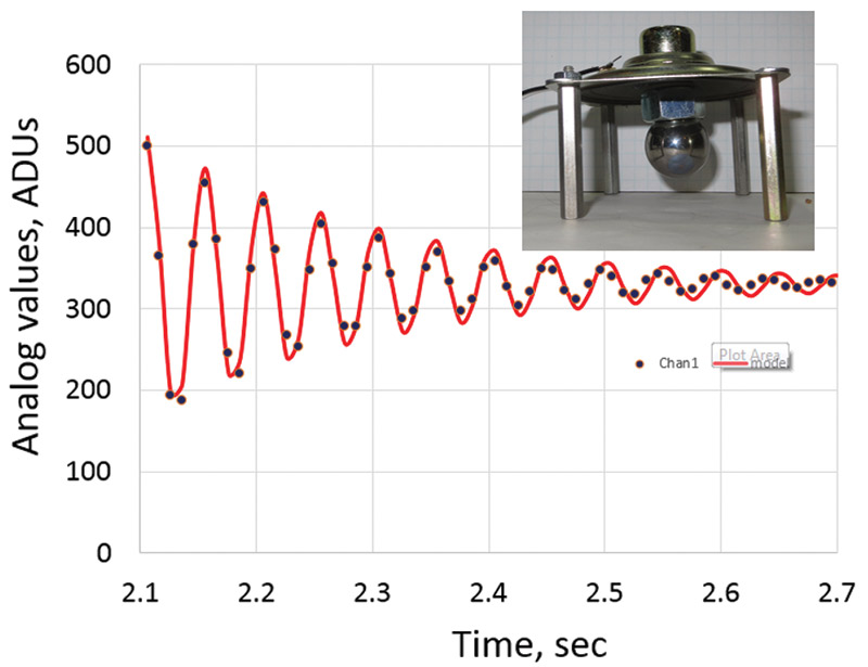
FIGURE 1. Measured response from the speaker and the fit to an ideal damped oscillator model. The agreement is excellent and even shows the onset of anharmonic behavior at small amplitude.
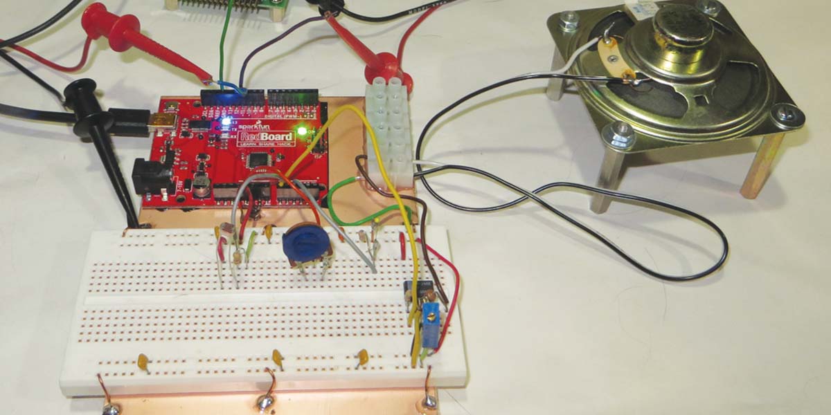
The setup for this measurement is shown in Figure 2. I used an analog front end to convert the induced current from the speaker into a voltage in the range an Arduino can measure with its analog pin.
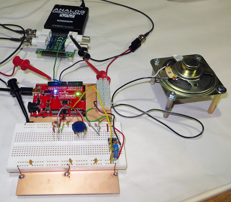
FIGURE 2. A complete measurement system consisting of the sensor (modified speaker), the analog front end (an op-amp mounted in a breadboard), the data acquisition system (my Arduino), and a scope used for diagnostics and debugging.
From the measured data, I can fit the resonant frequency and q-factor for an ideal damped oscillator. The agreement of this simple ideal model and this real physical system is really remarkable.
At the heart of this process is bringing the data into the computer. While there are a few really cool low cost data acquisition systems like the DATAQ DI-145 Electronic Strip Chart Recorder ($29) and the more advanced LabJack ($108), I’ve been exploring using an Arduino as a data acquisition interface to the real world.
Even a low end RedBoard (UNO compatible from SparkFun for $19.95) has six independent analog-to-digital converters (ADC), each with 10-bit resolution. This makes Arduinos potentially great platforms for sensor data acquisition. When I started down this path to use an Arduino as a data acquisition system, the stumbling block for me was how to get the data from the Arduino directly into an analysis tool like Microsoft Excel.
I wanted a method that was easy, robust, low cost, and wasn’t a long time-consuming process involving hacking a lot of code. Did I mention I wanted it to be easy?
The problem was not that I couldn’t find any way of doing this. The problem was that I found too many ways of doing this. When I Googled “Arduino data acquisition,” I got more than 250,000 entries. They generally fell into three categories: in real time through the serial port; data logging into an SD card; or by Wi-Fi into the cloud.
While data logging or sending the data to a cloud server are really cool, for my first application I wanted to use my Arduino as a tethered data acquisition unit and suck out the data over the USB cable. Programming the Arduino to print data to the serial port — while there are a few timing limitations — is easy. It’s getting the data from the serial port into an immediately useful format that was the challenge.
There were only 129,000 entries in Google under “Arduino serial data acquisition.” The options for reading the data on the serial port ranged from simple programs written in Processing, Python, or C, to using high-end tools like LabVIEW and MatLab. (Did I mention I wanted an easy process?)
Then, there were the stand-alone tools that folks had written to read the serial terminal, parse the numbers, and display them in various ways. Some were free; some cost from $19 to over $99.
I spent time playing around with many of these tools. My criterion was I wanted to look at the data in real time as it came out of the Arduino, and display it in a high quality plot — preferably Excel compatible. Plus, I wanted the learning curve to be at most five minutes with minimal additional code I had to add to my Arduino sketches. (Did I mention I wanted it easy?)
After trying out more than 20 different tools, I settled on the best tool I found that met my criterion of being really easy and — best of all — it was free: PLX-DAQ.
The Simplest Way to Get Data from an Arduino into Microsoft Excel
PLX-DAQ is really a macro that runs in Microsoft Excel. It is free and can be downloaded from Parallax, Inc. Ironically, it was originally written for Stamp microcontrollers — a competitor to Arduinos. Since it just reads the data coming in on the serial port, it’s really independent of the specific microcontroller, as long as the correct command words are sent over the USB bus.
The Arduino writes successive rows of data separated by commas to the serial port using the Serial.print () command. The word “DATA” has to be written in front of each row of data, with each column of data separated by commas. That’s it. That’s all that needs to be added to normal Arduino code to start plotting data in Excel using PLX-DAQ. Figure 3 shows a code snippet to write data to PLX-DAQ.
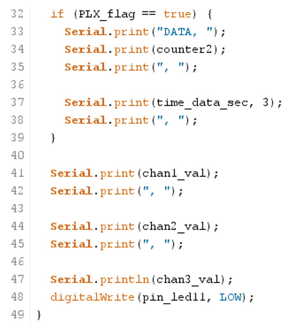
FIGURE 3. An example of the serial.print commands needed for PLX_DAQ to parse the characters on the serial port and place them in columns in a spreadsheet.
I added a conditional flag to print the first two columns of data containing the number of averages for each data point and the specific time the data item was taken, only when using PLX-DAQ.
Avoid this common problem: Only one device can use the serial port at a time. The most common mistake I make is having the serial monitor open to read the serial port while I want to have PLX-DAQ read the data. I get an error in this case. Wait for the code to be uploaded to the Arduino and be running. Make sure nothing else is talking over the same COM port, and then click the “connect” button. Likewise, to talk to the Arduino, be sure to click the “disconnect” button on the PLX-DAQ dialog box to free up the serial port connection for the Arduino.
As a quick test, I looked at the data printed to the serial monitor as the three channels were read and printed to the serial port. Figure 4 shows the serial monitor response — just as we expected. It has the right format to be read by PLX-DAQ.
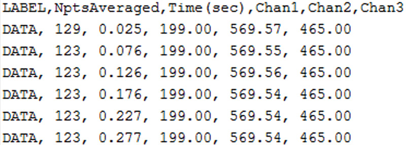
FIGURE 4. The characters printed to the serial port in the format read for PLX-DAQ to parse it into Microsoft Excel.
When you download and install the PLX-DAQ tool, it creates an Excel spreadsheet with an embedded macro. You have to enable the macro and allow it to run. The spreadsheet it opens up has three tabs, or worksheets. By default, PLX-DAQ will write all new data into the first worksheet. I set mine up to plot the values in the three data columns against the time column, using an X-Y scatter graph. This is just one of the multiple types of displays PLX-DAQ can create.
In the small dialog window that opens up in PLX-DAQ (shown in Figure 5), there are two settings you have to set: the COM port for the Arduino; and the baud rate. I always use the highest baud rate I can get away with. While most published example code I see uses 9600 baud, I never do this.
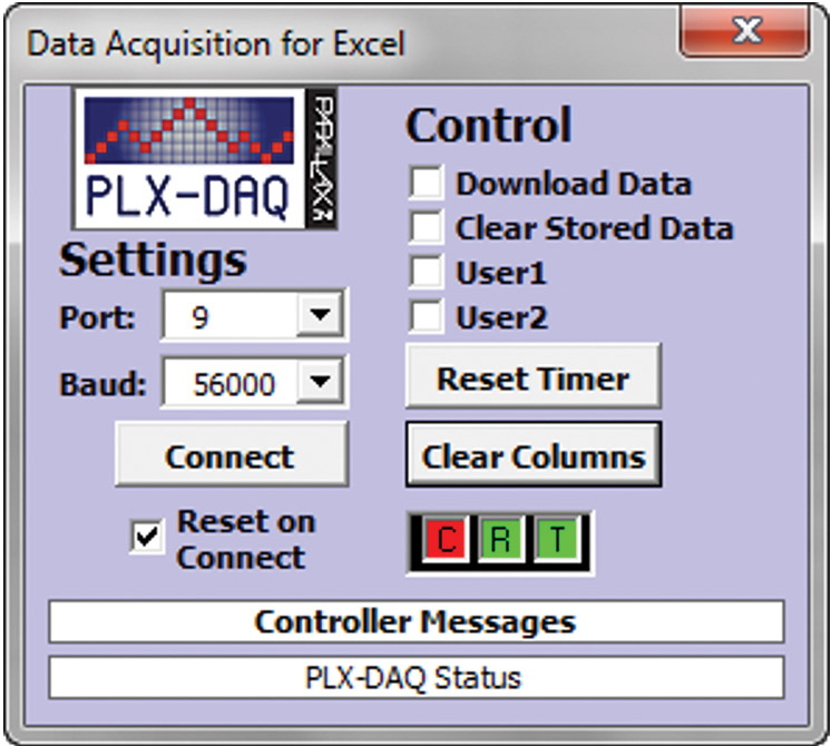
FIGURE 5. The dialog box to set up PLX-DAQ. It automatically opens when you open Excel and enable macros. You only need to change the COM port and baud rate.
The highest baud rate I routinely get transferring into PLX-DAQ is 56000. This is my default value. In the void setup() function, I place the line Serial.begin (56000);. You also have to set this value in the PLX-DAQ dialog box.
Avoid this common problem: While the standard baud rate for the serial port is 57600, PLX-DAQ only offers the option for 56000. If you use 57600, some of the data read by PLX-DAQ will be garbled. You must set up the baud rate in the Arduino sketch with the same value as you select in PLX-DAQ. I recommend the highest value of 56000 as your default.
When you click the “connect” button, PLX-DAQ sends a rest command to the Arduino which starts the sketch from the beginning and catches all the transmitted data. This is effectively the start button.
Figure 6 shows an example of the Excel spreadsheet with the five columns of data and the plot of the three analog channels. I created the plot using the built-in Excel functions so that any data written into the columns D, E, and F would be plotted in real time as it came in, using column B — the time — as the X axis.
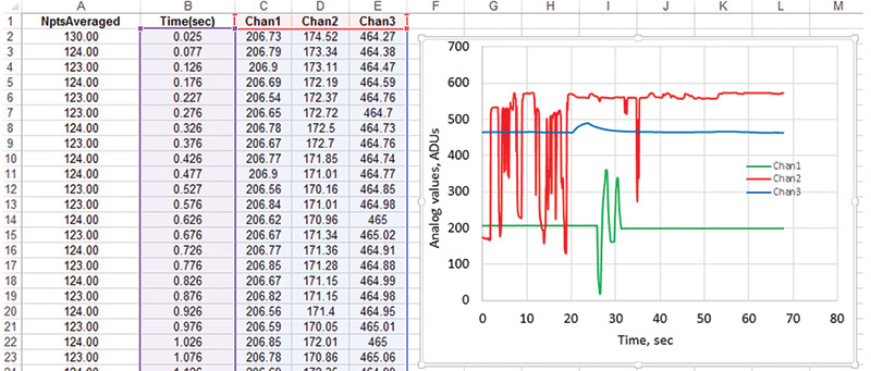
FIGURE 6. The final result: The spreadsheet showing the data as it came in and the resulting plot of the three channels of ADCvalues (0 to 1023) using the time stamp data. This plot can be modified using standard Excel tools.
A Little Finesse — Making Life Easier
It really took me less than five minutes after opening PLX-DAQ for the first time before I had data in Excel and plotted. Now, I was ready to add a few simple features to clean up the data.
PLX-DAQ understands a few code words. The word DATA in front of each line of data (separated by commas) is the command to place each data value in a separate cell on the same row.
The line feed Serial.println(), as the last line in the serial.print statements, also prints the line feed and tells PLX-DAQ to add the next set of data to a new row.
There are two other commands I find very useful. The first is CLEARDATA. When this key word is printed to the serial port, PLX-DAQ will clear the cells in the Excel spreadsheet and move its pointer to start adding data to row 1 in the first worksheet. This means I can use the same worksheet over and over again — especially if I have a graph already formatted the way I want.
When I have a set of data collected and I want to keep it, I make a copy of it and place the copy in the first sheet position. This is done with a right mouse click on the worksheet tab and selecting the copy command.
Avoid this common problem: Since the CLEARDATA command erases all the data in the spreadsheet, make sure you either want to remove the data or have a new worksheet set up in the first tab position before you click the “connect” button.
Now, I have a new worksheet ready to collect and plot data with formatted plots, but it’s full of old data. When the CLEARDATA command is sent, the old data in this new spreadsheet is cleared out and I start over with a blank worksheet. Fortunately, a plot is already formatted, waiting for new data to plot.
The second command that makes my life easier is LABEL. I like to have my data as well documented as possible. In this simple example, I wanted to display five columns of data, the number of points averaged per data value, the real time each data point was taken, and the three analog values from each channel. I used the LABEL command to send the labels for each column (separated by commas) as the first command.
This command only needs to be sent once, to set up the column labels. I put this in the void setup() function, so it executes right at the beginning of the sketch. Since I wanted a little flexibility on how I use the serial port, I added the flag to only print the LABEL command and values if the PLX_flag is set for true. These commands are shown in Figure 7.
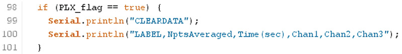
FIGURE 7. The additional commands added in the void setup() function to first clear the old data out and add labels in the first row of the spreadsheet.
With these two additional features, I can set up a worksheet exactly the way I want it with the graph formatted using all the built-in cool features of Excel, and I can use this worksheet over and over for each new run of measurements. The old data in the copied sheet is cleared out, the column headings are added, and all the data flows into the sheet in real time.
Measuring the Timing of Arduino Operations: a New Window for Debugging
Now that I could effortlessly bring data into a spreadsheet, I focused on the quality of the data and how fast I could take it.
A key feature of a data acquisition system is to have an accurate time associated with each data point. I didn’t just want a lot of data points; I wanted a lot of data at well-defined instants of time.
The best way of capturing the acquisition time is to take advantage of the built-in timer functions, millis() and micros(). They return the current elapsed time since the Arduino was turned on in milliseconds and microseconds, respectively.
As long as I record the system time just before and just after an analog measurement, I can get an accurate measure of the actual time stamp for each data point. The challenge was to determine how fast I could collect and write the data.
Avoid this common problem: Even if you initialize a timer as an unsigned long, the largest integer value it can hold is 4.3 x 10^9. If this is in microseconds, the longest time you can record before the timer resets is 4.3 x 10^3 seconds, which is about 71 minutes. If you want to record data with a time stamp for a longer time than 71 minutes, use the millis() timer. This can count up 1000x longer, or 49 days before resetting.
Most online forums suggest using the built-in timer functions like millis() or micros() to calculate the execution times and print the results to the serial port. You just have to add debug code to measure the time intervals between sections of your code, print the times out to the serial port, and read them with the serial monitor.
While this is a useful technique, I am a measurement guy and like to use my scope and digital write pins to get useful timing information of Arduino code. I think this is an important technique as it gives a very visual window into the time it takes for sections of code to execute. I use it to debug my code all the time.
My favorite scope is the Digilent Analog Discovery scope. This is a two-channel, 10 MHz bandwidth, 100 Msample/sec, USB scope with 14-bit vertical resolution and a built-in two-channel arbitrary wave generator. It also has a 16-channel logic analyzer. The user interface is incredibly easy to use and incredibly versatile, and at $279, it’s a steal.
The 10 MHz analog bandwidth is a perfect range for the Arduino. With this receiver bandwidth, we can see rise times on the order of 0.35/10 MHz = 35 nanoseconds. Figure 8 is a screenshot of the zoomed in rising edge of a toggling digital output pin on my Arduino showing a measured 10-90 rise time of about 16 ns — well below the estimated limit of 35 ns. Note that the acquisition rate is only 100 Msamples per second (or one sample every 10 ns), so there is a bit of interpolation used to get the 16 ns rise time. This is plenty fast for most analog applications.
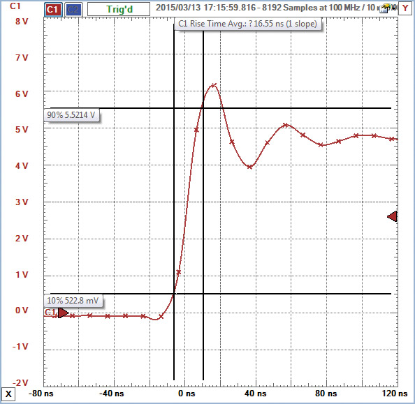
FIGURE 8. Screenshot from the Analog Discovery scope showing the measured 10-90 rise time of the Arduino digital signal of 16 nsec. This is limited by the scope. Its actual rise time, measured with a faster scope, is 3 nsec.
The RedBoard Arduino has an onboard 16 MHz clock generated by a very precise crystal. A single clock cycle is about 60 ns. In another experiment, I found that by using the PORTB command, I could toggle eight of the digital output pins off and on in four clock cycles, or in 250 ns. This sort of time is overkill for any typical data acquisition I had in mind, and I wanted to leverage the digitalWrite functions.
The first question I wanted to explore was just how fast can I toggle an output pin off and on using the digitalWrite command. I set up a sketch to just have the two commands digitalWrite(13, LOW) and then digitalWrite(13,HIGH) inside the void loop() function to turn output pin 13 off and then on. This code is shown in Figure 9.
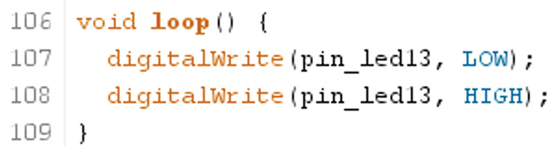
FIGURE 9. Code snippet to toggle pin 13 off then on as fast as possible.
I used the venerable pin 13 which also flashes the LED on the board. Figure 10 is a snapshot of the screen of the Analog Discovery scope showing the voltage at the output of pin 13. The pin is set low, then the next command is to write it high.
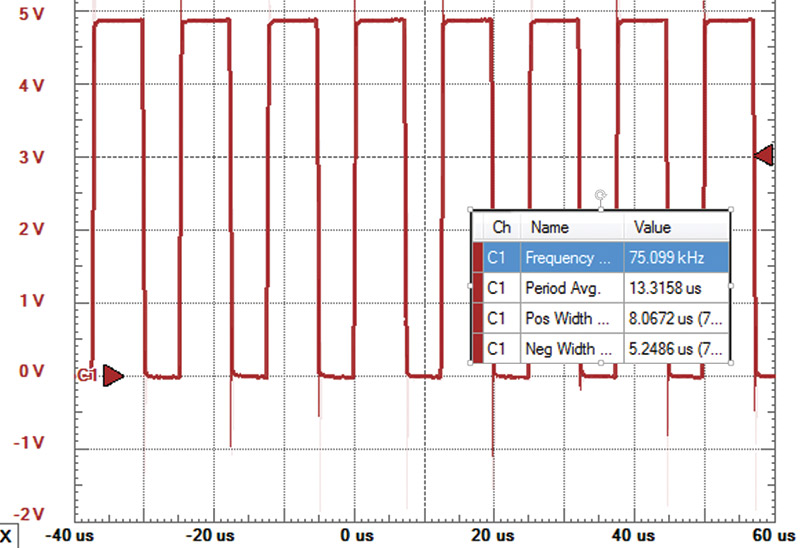
FIGURE 10. Screenshot for the Analog Discovery scope measuring the voltage on pin 13, showing the on and off time. Inset is the on-screen real time measurement of the waveform features.
In the scope trace, you can see the low lasts for 5.25 µs. This is about 90 clock cycles. Did I mention that the Analog Discovery scope also has over 50 math functions allowing high resolution waveform feature measurements? In this case, I extracted the off time and on time of the digital signal using a simple math function and displayed the extracted values in real time.
In this measured output, we see that the pin stays low for 5.25 µs, and then the output HIGH command is executed. This lasts for 7.18 µs, which includes the execution time for the loop command. Overall, this loop is executed in 12.43 µs. Altogether, this is about 200 cycles. This is plenty fast for my testing.
Adding comment lines to the code has no impact on the execution time. In fact, I wrote the toggle commands in a function and just called the function in the void loop() function. The execute time went up to 12.62 µs. This is only 190 ns of overhead to execute a function call, or about three clock cycles. Function calls are pretty fast.
We can use the overhead time as a starting place estimate; the overhead time to turn off pin 13 and turn it on, that’s about 12.4 µs. Now, we can start using it to help decode the timing for executing other functions like reading the analog pins and writing to the serial port.
How Long Does It Take to Read an Analog Pin?
I set up my initial experiments to read three analog channels. I connected some simple sensor inputs just so I had something fun to offer as signals. In channel 1, I had a simple one-turn pot connected between the +5 and gnd.
In channel 2, I had a thermistor connected to +5 with a 10K resistor. All resistors change their resistance with temperature. How much the resistance changes is described by the temperature coefficient of resistance (TCR). For a carbon resistor, it’s about 0.1% per degree C. A thermistor turns this problem into a feature. Its TCR can be as high as 5% per degree C.
The thermistor I used from SparkFun was nominally 10K ohms with a 5% change per degree C. Touching it increased its resistance by 20-40%. I turned it into a simple resistor voltage divider between +5 and gnd.
In channel 3, I added a simple light sensitive resistor, also from SparkFun. Its nominal resistance in the dark was about 10K ohms, and it could drop to 2K ohms in the light. Again, I just added it to a simple voltage divider and measured the voltage across the 10K resistor in series.
Using my digitalWrite triggers as a timer, I measured the time it took to read a single analog channel, and then to read all three channels sequentially. The code to do this is shown in Figure 11.
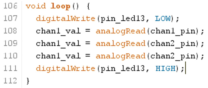
FIGURE 11. Code snippet to use the digital write pins as timers when reading three analog channels.
Reading one analog channel increased the time for the low signal to be on from 5.25 µs to 120.7 µs. This is about 115.5 µs for an analog read command. When reading three channels consecutively, the low bit time increased to 344.3 µs. Taking out the digitalWrite overhead, this is (344.3 – 5.25)/3 = 113 µs per channel — very close to the measurement of the single analog read. To be generous, I use the value of 120 µs as the time to read an analog channel.
In principle, if there are no other functions going on, it sounds like I could take one channel’s worth of data at a sample rate of about 8 kHz. However, it’s what we do with the data that will really slow things down.
How Long Does it Take to Perform a Serial.print()?
For this first data acquisition system, I wanted the fastest data acquisition I could easily get and have the data go into an Excel spreadsheet with PLX-DAQ. The limitation I quickly found was the print command to the serial bus.
The first way to decrease the time to print to the serial bus is to use the highest baud rate practical. The difference in times to print using 9600 and 56000 is almost (but not quite) the x5.8 difference in baud rate. There is some overhead used in the serial.print command.
Printing one character at 56000 takes about 0.4 ms. However, printing 30 characters takes about 5.6 ms. Depending on the number of characters in the data being printed, the total print time in my code may vary from 2 to 7 ms. This means that a safe sample interval is 8 ms.
Getting the Most Out of the Measurements by Averaging
Based on the variation in the time for the print command, I decided to use a short sample interval of 10 ms. This was reasonable for my typical application and also robust, leaving plenty of time (even in the worst case) for the serial.print command to execute.
If the print command took only a few ms, this left a lot of dead time. I decided to take advantage of this by using the available time in the sample interval to repetitively read the analog channels and average the results. What is exported to the serial.print command at the end of each time interval is the average of all the readings during the interval.
When the time available to sample was on the order of 7.5 ms and it only took about 0.33 ms to read the three channels, it was possible to perform as many as 7.5/0.33 = 20 readings for each exported data point. This helps reduce the noise.
I used output pin 12 to toggle on when I started to read the first analog channel and toggle off when I finished reading the last channel. I used pin 11 to turn on when I started the serial.print operations and toggle off when I finished. Figure 12 shows the measured timing diagram when the sample interval is 10 ms.
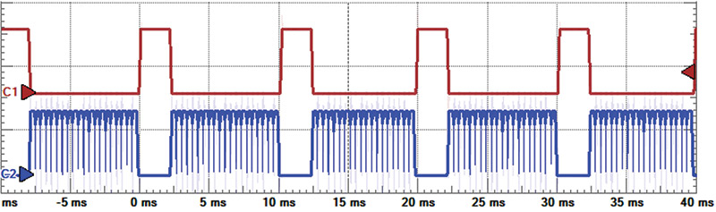
FIGURE 12. Measured timing diagram showing the relative time to print to the serial port (top trace, on time) and the successive analog channel reads (bottom trace, on times). This shows the many consecutive analog reads which were then averaged to arrive at one value per channel in each sample interval.
Conclusion
I like data and I like easy. I started this project with a goal to find a simple, robust, and easy way of bringing data from my Arduino into Microsoft Excel. After a lot of evaluation, I decided on PLX-DAQ as the tool to read data on the serial port directly into Excel. This turned out to be a perfect solution.
Along the way, I found that a valuable debug tool was to use a few digital write pins as a new window into the timing associated with different functions. This gives a quick graphical view of when the code executes operations and how long it takes.
This solution turns the very low cost Arduino into a very robust, versatile, and accurate data acquisition system capable of as fast as 100 points/sec, plotted directly into Excel in real time. It’s a great starting place to feed my need for data. NV
Links
www.dataq.com/products/di-1100/
http://labjack.com/u3
www.sparkfun.com/products/12757
www.parallax.com/downloads/plx-daq
Digilent Analog Discovery: https://bit.ly/3XVIT50
www.sparkfun.com/products/250
www.sparkfun.com/products/9088
Downloads
What’s in the zip?
Source code for PLX-DAQ Example