There has been a lot written about the design and implementation of digital filters over the years and I periodically survey the literature to try and keep up with it. It seemed the right time to look around again when I decided to build a digital color organ [1] which would require digital filtering. During this latest survey, I came upon Lattice Wave Digital Filters (LWDFs) which I was not familiar with. These filters piqued my interest as they had intriguing properties directly applicable to my application.
Typically, when I find a technology that interests me, I go overboard in my research and spend lots of hours playing with it in order to understand it. LWDFs were no exception. This article, and the accompanying design tool, were a result of my investigation into LWDFs which were just too cool to pass up. We will get to LWDFs shortly, but first a little context.
Digital Filters
There exists two major classes of digital filters referred to as Infinite Impulse Response (IIR) — sometimes called a recursive filter — and Finite Impulse Response (FIR) or convolution filters. Both of these filter types have advantages and disadvantages which make them each suitable for a variety of applications.
IIR filters might be used, for example, in applications where cost is a concern because they can be implemented using a minimum of hardware/software resources. FIR filters would be used in applications where linear phase response is required such as in high end audio applications, the processing of sensor data, or possibly radio telescope data. FIR filters use more resources to implement to the same order as an equivalent IIR filter.
Typically, IIR filters are not as stable as their FIR counterparts. This fact is reflected in their names. Infinite Impulse Response filters will typically ring for a period of time after being subjected to an impulse waveform. Finite Impulse Response filters are better damped and any ringing of the filter will be of much shorter duration.
IIR filters also have sensitivity to word length limitations and coefficient round off errors which makes their implementation tricky. All this is to say that testing is very important for any digital filter you design (regardless of topology) to make sure it is performing per your requirements.
IIR filters were appropriate for the application I had in mind because of their inherent efficiencies, but only if their stability issues could be controlled or eliminated. This is where LWDFs came into play.
All of the information I found on these filters indicated they were extremely stable, had a large dynamic range, and weren’t sensitive to either limited word lengths or round off errors. LWDFs don’t correct the erratic phase response of classic IIR filters but phase response is not important in my application.
LWDFs were first proposed by Professor Alfred Fettweis in 1971 and are backed with an extensive amount of complex network theory which one does not need to understand to apply. A lot of information can be found on the Internet describing these filters. The Resources sidebar details some of the most useful papers I found. Specifically, the TI application note and the paper by Gazsi were the most helpful to me and my understanding of this technology.
LWDFs are a cascade of first and second order all pass filter sections. Each all pass section is made up of a two port adapter (picture a little box with two inputs in1 and in2 and two outputs out1 and out2) along with a one sample delay element. Every adapter has a gamma value (gamma values range in value between -1 and +1) which controls the response of the all pass section. Adapters are implemented in software using a set of network formulas which require a single multiplication and three additions each.
The LWDFs we are discussing use four types of adapters as filter building blocks. The number and the variety of adapters used along with the gamma values associated with each are typically generated using some sort of filter design tool. (More on filter design tools shortly.)
Even though the gamma value controls the response of the all pass sections, we don’t typically deal directly with gamma in an implementation. Instead, alpha values in the range 0 to 0.5 are used as multipliers because they are easier to use and implement. Each of the four adapter varieties uses a different method of converting gamma into alpha. This is illustrated in Table 1.
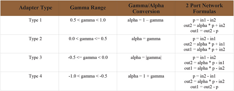
TABLE 1
Low pass, band pass, band reject, and high pass filters of Butterworth, Chebyshev, and Cauer Parameter (Elliptic) forms can be built using the adapter building block approach. Actually, only low and high pass filters are directly implemented. Band pass and band reject filters are produced by cascading high pass and low pass filters together.
Note that only odd order (first order, third order, fifth order, etc.) filters can be designed using these techniques. Note also that there is a one-to-one ratio between filter order and the number of adapters necessary to achieve it. Three adapters will be required for a third order filter, for example.
Adapters and delays are connected together using a standard topology to form LWDFs. The standard topology is shown in Figure 1.
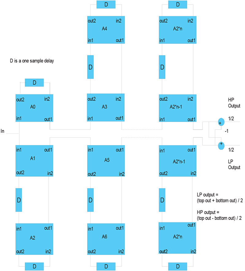
FIGURE 1
The single sample delay associated with each adapter records the previous output of the adapter. The previous output is used in conjunction with the current input and gamma/alpha value to produce a new output from the adapter. All adapters working together form the LWDF.
As also shown in Figure 1, the filter’s response is determined by how the final top and bottom adapter output are combined. If the top and bottom outputs are summed and divided by two, the result is the low pass response. If the bottom output is subtracted from the top output and divided by two, the result is a high pass filter.
Band pass and band reject (also called band stop or notch) filters are built by cascading a high pass LWDF and a low pass LWDF, in that order. If the low pass output is used from the final low pass filter, a band pass filter results. If the high pass output of the low pass filter is used instead, a band reject filter results. Of course, it is necessary to design the high and low pass filters correctly to get the band pass or band reject response you desire.
The order in which adapters are executed is very important to the stability of the resulting LWDF. It is important to execute all of the top adapters (A0, A3, A4, etc.) before executing the bottom adapters (A1, A2, A5, A6, etc.). Also, the adapters must be executed from the outside in. That is, A2 is executed before A1, A4 before A3, etc. The following example illustrates this.
LWDF Design Example
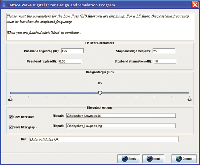
Suppose we want to design a filter with the following characteristics:
- Sample rate: 16,000 samples/second
- Type: Chebyshev Low Pass
- Passband edge frequency: 125
- Stopband edge frequency: 250
- Passband ripple (dB): 0.5
- Stopband attenuation (dB): 18
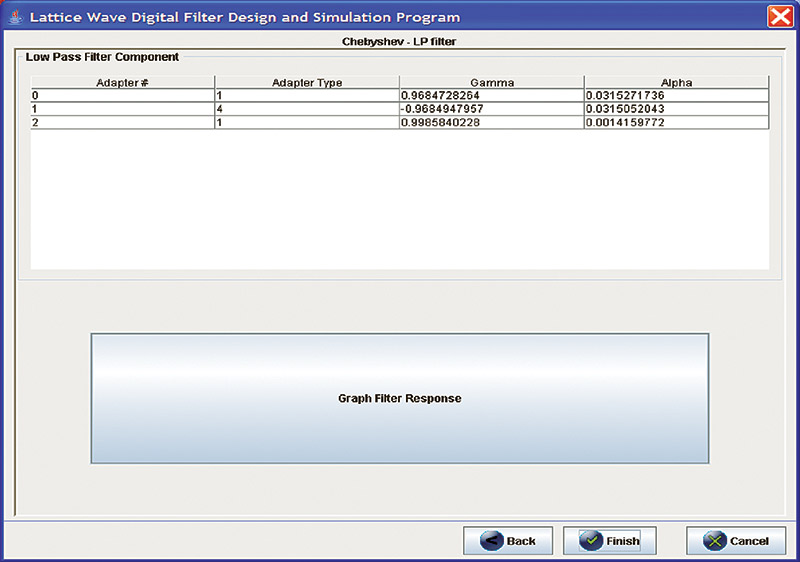
Running these specifications through an LWDF design tool tells us that the resulting filter will be third order. Figure 2 shows us what the actual filter topology looks like.
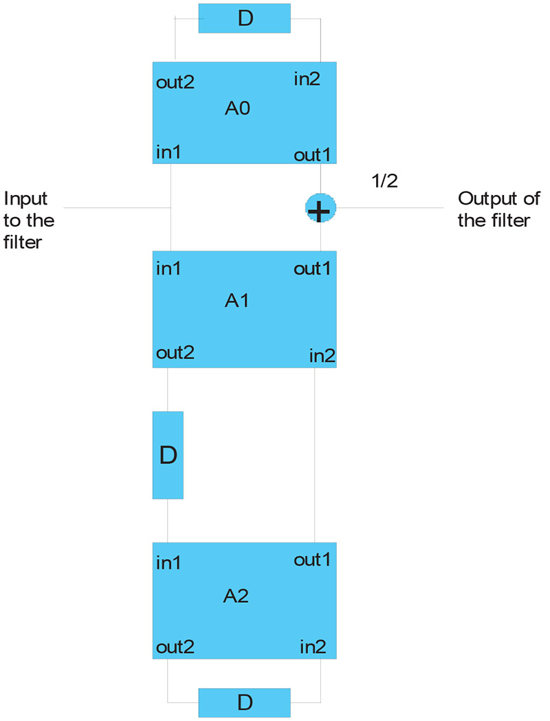
FIGURE 2
In addition to the filter’s order, the LWDF design tool provides us with information about the types of adapters to use and the gamma/alpha values associated with each. For our example filter, see Table 2.
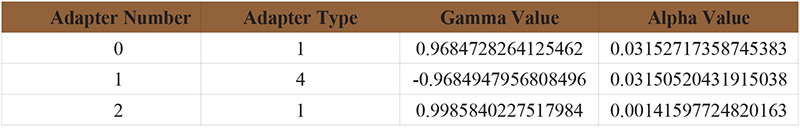
TABLE 2
With this information, the filter can be implemented. Listing 1 shows a Java implementation, though you could implement it in the computer language of your choice. If you fed this function a stream of appropriate digital samples, you would get a response close to what was specified.
Listing 1
/**
* Listing One – Java implementation of Low
* Pass Lattice Wave Digital Filter
*
* Third order Chebyshev with fc ~ 125 Hz
*
* Adaptor 0 Type 1
* Adaptor 1 Type 4
* Adaptor 2 Type 1
*
* Adapter implementation order: 0,2,1
* The three delays are integer values declared
* elsewhere
* @param sample the input sample to the filter
*
* @return filtered output sample
*/
public int filter(final int sample) {
// Alpha values for Low Pass filter
double ALPHA0 = 0.03152717358745383;
double ALPHA1 = 0.03150520431915038;
double ALPHA2 = 0.00141597724820163;
// Adaptor 0 - Type 1
int in1 = sample;
int in2 = delay0;
int p = in1 - in2;
double acc = p * ALPHA0;
int out2 = (int) acc + in2;
delay0 = out2;
int out1 = out2 - p;
int topOutput = out1;
// Adaptor 2 - Type 1
in1 = delay1;
in2 = delay2;
p = in1 - in2;
acc = p * ALPHA2;
out2 = (int) acc + in2;
delay2 = out2;
out1 = out2 - p;
// Adaptor 1 - Type 4
in1 = sample;
in2 = out1;
p = in2 - in1;
acc = p * ALPHA1;
out2 = (int) acc - in2;
delay1 = out2;
out1 = out2 - p;
int bottomOutput = out1;
// Combine outputs
return ((topOutput + bottomOutput) / 2);
}
Assembly language programmers don’t get off so easy. Listing 2 shows the same filter written in MSP430F2012 assembly language. (Listing 2 is available in the downloads at the end of this article.)
LWDF Design Tools
When I first started experimenting with LWDFs, I used a program called wd_coeff.exe from TI (see Resources) to generate adapter types and alpha values for the filters I needed to build. I then hand-coded the filters in MSP430 assembly language and generated a series of sine waves (internal to the processor) to validate my designs. This was a tedious process to say the least. Later, I wrote a Java program to simulate the filters with the coefficients generated by wd_coeff.exe. This was better, but still left a lot of room for error. Finally, I wrote a full LWDF design program called LWDFDesigner.java that takes a set of filter specifications like we used for our example and does the following:
- Performs the LWDF calculations necessary to design the filter. LWDFDesigner supports Butterworth, Chebyshev, and Cauer Parameter (Elliptic) filters of low pass, band pass, band reject, and high pass varieties.
- Compiles the filter design into a filter topography in memory.
- Subjects the compiled filter to a stream of digital samples from 50 Hz to 50 Hz less than one half the specified sample rate, and captures the results.
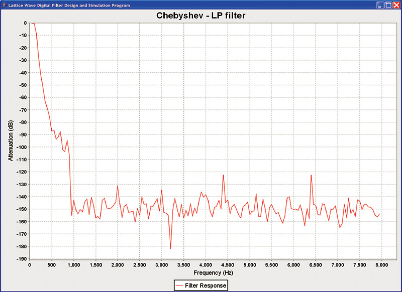
- Analyzes the filter’s response and graphs the result.
LWDFDesigner makes LWDF design easy. The ability to see the results of filter execution immediately takes most of the guess work out of the process. LWDFDesigner is still a work in progress and will evolve over time. I plan on adding a plug-in to the program that will generate the MSP430 assembly code for the filters directly. As it stands now, the filters designed using LWDFDesigner must still be coded by hand using the information generated by the program.
The Design Cycle
I would like to tell you that by using a LWDF design tool you are able to crank out filters that match your specifications exactly every time, but I cannot. I know from implementing LWDFDesigner that inside these design programs are approximations and parameter quantizations that result in a filter that, in most cases, is close to what was specified. In fact, both the TI program and LWDFDesigner support the concept of design margin which has direct impact on the designed filter.
Design margin is a number from 0 .. 1 which determines whether the filter’s stopband or the passband should be given the most effort to get right. Values towards one concentrate the design accuracy on the passband. Values towards zero concentrate on the stopband. Tweaking the design margin just a little bit changes the generated gamma values; sometimes by quite a bit.
With these facts in mind, the LWDF design cycle looks something like this:
- Determine the initial set of filter specifications for the filter you want to design.
- Run LWDFDesigner inputting these specifications.
- Graph the result to see the resulting filter response.
- If the filter matches your specifications, you are done with the design phase. If not ...
- Modify one or more of the filter’s parameters and/or the design margin and go back to Step 2 and try again.
Once you are satisfied with the design, it is time to implement the filter. If you are a C or Java programmer, you can write code that looks like Listing 1, making sure you code the correct adapter types and gamma/alpha values produced by the design tool. Remember also it is very important to implement the top adapters first and get their execution order correct. If you are an assembly language programmer, you can take the alpha values and run them through Horner.java provided with my article in the September ‘07 issue to get the equations and/or the code for incorporating into your filter.
Conclusions
LWDFs are a good choice for many applications. They are easy to design, for the most part they function as designed, they can be implemented in a small amount of data and code space, they use CPU cycles sparingly, and seem to be stable. Maybe you can put them to use in your next project. NV
Running LWDFDesigner.java
To run LWDFDesigner.java, you will need to have a Java Development Kit (JDK) installed on your computer. The program was written for use with Java 5 which is available for free from Sun Microsystems at http://java.sun.com/javase/downloads/index_jdk5.jsp. Version 6 of Java should also work.
An executable version of the LWDFDesigner.java program is available in the downloads and is named LWDFDesigner.jar. The code is meant to be run directly from the jar file using the following command line from a command shell (cmd.exe) in Windows XP:
java -jar <path to where the jar file resides>\LWDFDesigner.jar
If this doesn’t work, make sure the bin directory of the JDK installation is on the Path in your command shell. Alternately, you can change directories to the JDK bin directory and run the above command from there. LWDFDesigner does not require any command line arguments.
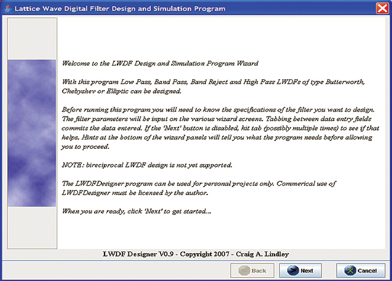
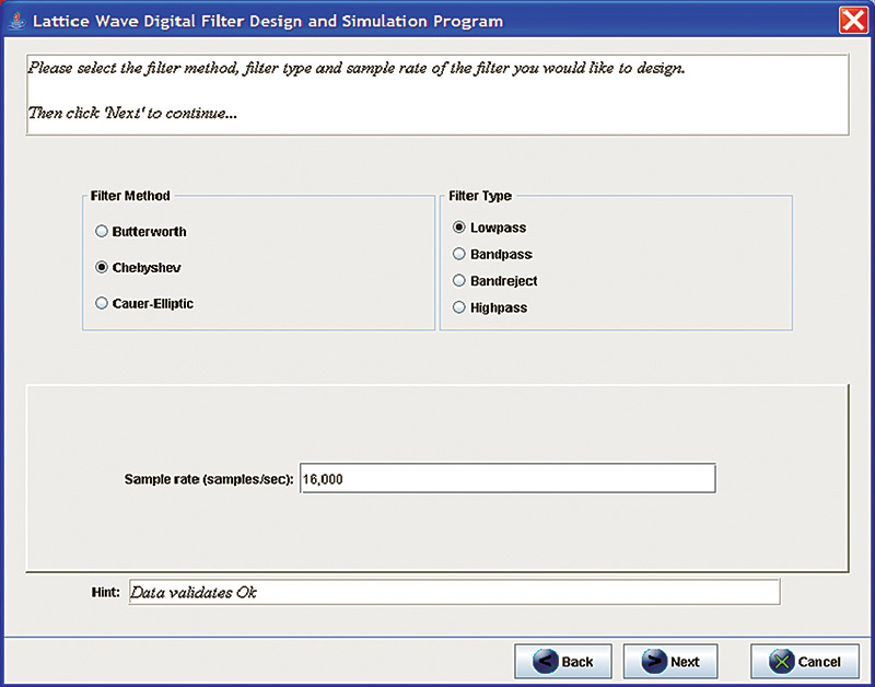
LWDFDesigner is written as a graphical-based wizard that guides you through the steps necessary to successfully design a filter. Each wizard page or panel validates the user entered data before allowing the user to proceed to the next page/panel. As you enter data into the program, you should tab between fields to commit and validate data. When the program is satisfied with the entered data, the ‘Next’ button will be enabled allowing you to move to the next page. The screenshots shown give you an idea of what to expect.
Resources
You may find the following resources helpful:
Java version 5 is available at: http://java.sun.com/javase/downloads/index_jdk5.jsp.
A Texas Instruments application note discussing Lattice Wave Digital Filters is available at: http://focus.ti.com/mcu/docs/mcusupporttechdocsc.tsp?sectionId=96&tabId=1502&abstractName=slaa331.
Fettweis, Alfred, “Wave Digital Filters: Theory and Practice”, Proceedings of the IEEE, Vol. 74, pp. 276-327, February 1986.
Gazsi, Lajos, “Explicit Formulas for Lattice Wave Digital Filters”, IEEE Transactions on Circuits and Systems, Vol. 32, No. 1, pp. 68-88, January 1985.
Footnote
[1] A color organ is a device that splits music up into numerous frequency bands and modulates colored lights (one color of light per band) according to the musical content.
Downloads
Code listing 2 and LWDFDesigner.jar