What is noise? We all experience it and generally want to avoid it. Noise is usually an unwanted signal, and is the combined effort of every other signal trying to compete with one another. Think of when you are at a party or out at dinner in a restaurant and you have to talk louder just so that the people at your table can hear you. By talking louder, you have increased your signal-to-noise ratio by increasing the signal strength directly at the source. So, what if your output level or source signal is at a fixed volume or strength and you can't go any stronger? Then what?
One method is to repeat yourself so the person you are directing your conversation to can understand what you are saying. This amounts to transmitting the same data several times. This may improve the signal-to-noise ratio, but the rate of data then goes down as a consequence. What you have done and may not have even realized it is called ensemble averaging.
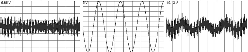
If you consider noise to be random in nature and it is combined with your true signal, then repeating yourself has a tendency to keep the random noise at a constant level while reinforcing the true signal embedded within the noise. For every time that you have to repeat yourself — or in terms of electronics, “transmit” — your signal-to-noise ratio improves on the receiving end, and can be referred to as the square root of the number of samples “N” (Figure 1), or the number of times you said the same thing over:
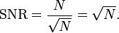
FIGURE 1.
So, for example, if you had to repeat yourself twice, the signal-to-noise ratio would be 1.414-to-1. Likewise, if you had to repeat yourself three times, the signal-to-noise ratio would be 1.732-to-1. After the third time, I usually won’t repeat myself with the exception of telling one of my daughters something I know they heard the first time. (That, however, is another topic.) This method only works if you have the luxury of a signal that does repeat and the data rate is low. Using two or more sensors to receive the same signal can circumvent the need to read the signal over several times, but in practice may not be practical because of the physical redundancy in board real estate that the design requires.
There is a derivative of ensemble averaging that can be applied physically that avoids having to sacrifice the data rate called differential signaling. Instead of reading the signal twice, two sensors are used differentially to one another. This method has the ability to mathematically cancel out most of your common mode signal (or noise) and provide a greater signal-to-noise ratio than just taking two samples and summing them together because while the signal increases, the noise floor is suppressed due to common mode rejection.
Honestly, I wish this method received more attention in some of the basic text books in schools. Many times, a book will cover a topic on how to read one sensor and simply move on without discussing the benefits one can gain from using two sensors together instead. This method is commonly used in data communication such as Ethernet, RS-485, etc., where the data being sent uses two signal lines that are 180 degrees out of phase. Differential signaling, however, is not limited to digital applications. It has been used for years in the audio industry, specifically for long lengths of microphone cables to balance out any electrical noise the cables — acting as an antenna — could pick up.
Differential signaling can be used for light sensors, sound applications, radio, accelerometers, gyros, and much more. For a thought exercise, think about what results you might get with two accelerometers mechanically locked together on a fixed plane and reading the signals from each of them differentially. As they move together, the signals would cancel out, but what if you pivoted one accelerometer on the Z axis with relation to the other one? What kind of signal would you see then? The signal would be similar to that of an angular rate gyro derived from using two accelerometers differentially that were mechanically locked to the same plane.
However you decide to use two identical sensors differentially, one sensor — if not used 180° out of phase — is used as a reference and the other sensor is used as the actual input. Referring again to the noisy restaurant scenario, slightly turning you head towards someone allows you to hear them better. We could argue the reasoning is that one ear is simply closer now to the source, and while some of that would certainly be true, your brain is a remarkable filter and there is more differential sensing and filtering going on than you might realize.
If the ambient noise is allowed to target both sensors (ears) simultaneously, then looking at the data from the sensors differentially will cause the ambient noise to mathematically cancel out leaving only the true signal if one sensor is positioned slightly closer to the source than the other.
In Figure 2, the top and middle graphs represent the left and right channels with significant noise added. If you look closely, you can see slight variations between the two. The bottom graph in Figure 2 represents the difference or differential between the left and right channels as a nice sine wave. Notice that all of the common mode “noise” present in the left and right was canceled out.
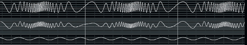
FIGURE 2.
A practical circuit application of the above description would be for a microphone to block out any loud ambient noise, such as a plane or simply a windy day. The circuit in Figure 3 will do just that. In this configuration, the LM1458 dual op-amp creates a differential input with a balanced load on each input. This way, the inputs electrically “see” the same load, which is important for making this kind of differential measurement.
FIGURE 3.
The microphones should be placed close to one another and will exhibit a pickup pattern that resembles a bidirectional microphone (see Figure 4) where one lobe is additive (non-inverting) and the other lobe is subtractive (inverting). In the mid-region is a dead zone where the input from each microphone cancels out any common mode signals.
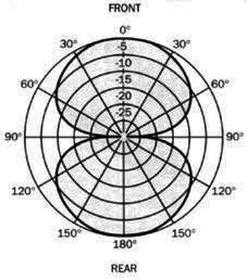
FIGURE 4.
A method to improve the signal-to-noise ratio (adopted from early radio) is to use a regenerative circuit or Q-multiplier circuit. This method is essentially an active filter that reinforces itself with positive feedback. A small portion of the input signal is amplified and fed back into the input in a positive reinforcing way. This has the effect of attenuating any noise while at the same time re-enforcing a signal hidden within the noise. A transistor with a normal gain of 10 or so can have a perceived gain of 10’s of thousands if applied in a regenerative circuit correctly.
Another method — again, adapted from early to more recent radio — is to use a local oscillator and mixer to level shift the input signal to another frequency band. This method is especially nice if you want to remove most (if not all) of the low frequency noise interference associated with 50/60 Hz, fluorescent lighting, etc., and create a final output signal with an exceptionally low noise floor.
Mixing is usually reserved if you have a particular target frequency that you are interested in. How it works is by literally mixing two signals together, which include the frequency that you are interested in plus a local oscillator frequency. Say, for instance, that you want to listen to 100.5 MHz on the FM dial (refer to Figure 5). Without knowing it, you are actually tuning the local oscillator to 89.8 MHz ... the reason will be explained later.
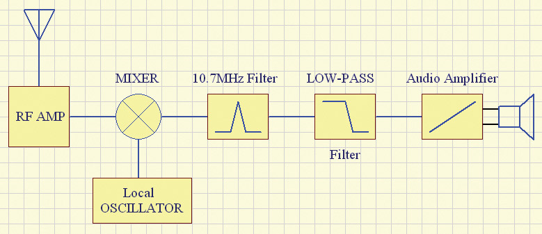
FIGURE 5.
When you combine two frequencies, you get those two frequencies, but you also get their sum and difference derivative frequencies. So, for 100.5 MHz and 89.8 MHz, you not only get those two frequencies, but you also get 10.7 MHz and 190.3 MHz. The radio industry has standardized a specific filter frequency for both FM and AM radio which happens to be 10.7 MHz for FM and 455 kHz for AM. Because the example radio station is FM, the 10.7 MHz filter is of importance here.
What this filter does is eliminate everything but the 10.7 MHz frequency, allowing only that frequency to pass. Since that frequency is only produced in the receiver circuit if your target frequency is present and agrees with the local oscillator frequency, it can be said that if 10.7 MHz is present or detected at all, then you are “tuned” to your target frequency or that the target frequency is present somewhere within the received signal.
Next — and this seems counter-intuitive — is that we remove the 10.7 MHz signal we just tuned to by using a low-pass filter. What this does is not only eliminate the 10.7 MHz signal we just filtered, but by passing it through a low-pass filter we are left with the low frequency modulated data originally transmitted from the radio station. This can be audio data, digital data, etc. For standard FM radio, there are a few more filtering processes that need to take place, such as decoding the left and right stereo, etc. Hopefully, the idea here is more on how to detect and isolate your signal from the noise. A similar technique can be applied to ultrasonic, IR, etc., and does not necessarily need to be confined to radio. I have used this technique on RFID tags and some ultrasonic applications, as well as rolling my own IR receiver for a non-standard modulation frequency. NV
References
Signal-to-noise ratio http://en.wikipedia.org/wiki/Signal-to-noise_ratio
Shot noise http://en.wikipedia.org/wiki/Shot_noise
Ensemble averaging http://en.wikipedia.org/wiki/Ensemble_averaging
Regenerative circuit http://en.wikipedia.org/wiki/Regenerative_circuit
Microphone basics www.ccisolutions.com/StoreFront/category/microphone-basics-part-2