Impedance matching is not mysterious, it is really just about controlling reflections
My previous article on transmission lines (a.k.a., feed lines) and standing wave ratio (or SWR) explained how RF energy travels in the line and what happens when it encounters a load or different type of line. The resulting reflections create standing waves of voltage and current, just as water waves do when they encounter an obstruction. As mentioned last time, the RF energy bouncing around in the line can create problems with digital signals and can result in extra losses.
This time, we’ll take a look at several techniques for dealing with the reflections and how the same techniques are used in circuit design. This is called impedance matching.
Review of Reflections
No matter what kind of wave we are talking about — electromagnetic (EM), acoustic, or ripples on a rope — whenever the wave encounters a change or discontinuity in the impedance of whatever medium it’s flowing in or on, the wave’s components have to change as well. For example, if we connect a 50Ω RG-58 cable to a 75Ω RG-6, the electric and magnetic field components of the wave change at the junction of the two cables. The change in impedance is called a mismatch.
To create the abrupt change, the wave splits into two new waves traveling in opposite directions but with the same total amount of energy. One wave travels into the new medium (the forward wave) and the other wave goes backward in the old medium (the reflected wave). The larger the discontinuity, the more energy remains in the reflected wave.
If the new medium’s impedance is zero (a short circuit) or infinite (an open circuit), no energy is transferred into the new medium; all of the energy is reflected and the SWR is infinite. The wave is reflected again at the source and heads back in the original direction. The split-and-reflect process occurs at the discontinuity on every round trip. As the reflected wave travels back and forth, some of that energy is lost through resistance (for an EM wave) or friction (for a mechanical wave) along the way. (The video “Similarities in Wave Behavior” referenced in the previous article at www.youtube.com/watch?v=DovunOxlY1k shows this process clearly.)
Imagine an RF signal from a transmitter in a piece of coaxial feed line connected to an antenna. Now, break up that RF signal into a sequence of packets, like boxcars on a train. Figure 1 shows one such packet as it bounces back and forth, getting smaller and smaller as it transfers power to the antenna, and loses power from losses in the cable.
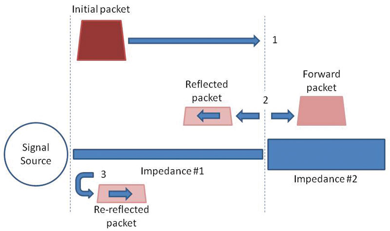
FIGURE 1. A packet of RF energy from the source travels to the end of the transmission line (1) with impedance #1 where it encounters transmission line with impedance #2. The packet splits (2) into a forward packet continuing on and a reflected packet headed back toward the source. At the source, the reflected packet is re-reflected (3) and the process repeats until all of the packet energy has been transferred to the second line or dissipated as heat.
If the packet has a very short duration and you looked at it on an oscilloscope, you would see it coming and going with its shape determined by the various discontinuities in the feed line. In fact, that is exactly what a time-domain reflectometer (TDR) does: Generate a sharp pulse in the line and display it. The shape of the returned pulse and the time it takes to make the round trip show just where the discontinuity is and its impedance.
To an RF engineer, the reflections dissipate signals as heat in the feed line, create excess voltages and currents, and alter impedances. To a digital designer, the reflections on a printed circuit board (PCB) signal trace can distort rising and falling edges of digital pulses, creating false clocks, delays, and erroneous values. As clock speeds rise and transition times fall, eliminating these reflections can become quite important to reliable operation.
There are several ways of eliminating the reflections. Some work at a single frequency, and some over a wide range of frequencies. Some use electronic components, and some can even be constructed from more transmission line. Let’s meet a few of the more common tricks of the trade for impedance matching.
Resistive Impedance Matching
One of the simplest ways of getting rid of the reflections is to simply dissipate them as heat with resistors. The result is that the source of power is happy with its load, the output circuit is happy with the power delivered, and both are relatively isolated from the effects of the other. This isn’t impedance matching as much as it is “impedance hiding,” but the net result is the same: No reflections.
Figure 2A shows a resistive T attenuator used to match impedances. The goal is to make the load presented to the signal generator close to 50Ω, no matter what value ZIN of the Circuit Under Test (CUT) may be. In the process, however, the attenuator knocks the input signal power down by a factor of 10 (10 dB)! This only works if you have power to spare from the source.
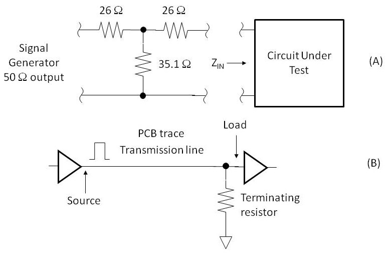
FIGURE 2. At A, a 10 dB attenuator insures that the signal generator output load is between 40.9Ω and 61.1Ω — no matter what load the CUT presents. This is useful in stabilizing the generator output as the circuit is adjusted. At B, a terminating resistor is used to make sure no reflections are generated when the pulse traveling along the PCB trace transmission line encounters the logic circuit's input.
If ZIN = infinity (an open circuit), then the generator “sees” the 26Ω and 35.1Ω resistors in series for 51.1Ω, and an SWR of 51.1/50 = 1.022. If ZIN = 0 (short circuit), the input impedance is 26 + 35.1 // 26 = 43.9Ω for an SWR of 50/43.9 = 1.14 (// means “in parallel with”). Any other impedance will present a load between 43.9Ω and 51.1Ω, so the generator’s output will not be greatly affected by ZIN.
Many test setups specify attenuators at the output of signal generators. It’s not because the generators are putting out too much signal; it is to present a stable impedance to the generator to avoid having to constantly readjust for a constant output level as a load changes.
Digital system designers can use resistors to terminate a PCB trace carrying high speed signals as shown in Figure 2B. The resistor is connected to common at an IC input. The termination makes sure no reflections are generated to travel back and forth on the trace. Each logic family has techniques for controlling reflections on signal lines. Check the datasheets for information on terminations and working with high speed signals.
Microstrip Transmission Lines
Every signal-carrying PCB trace is a transmission line. For high speed signals, treating the traces as microstrip transmission lines helps avoid erratic operation from reflections. Microstrip is formed when a trace runs over or between ground planes — a common situation on multi-layer boards. You can learn more about microstrip at www.microwaves101.com/encyclopedias/microstrip and the Analog Devices tutorial “Dealing with High Speed Logic” (www.analog.com/media/en/training-seminars/tutorials/MT-097.pdf) is a good introduction.
Mechanical Impedance Matching
A less wasteful method of getting rid of the reflections is to transform the mismatched impedance to a different value that doesn’t cause reflections at all. The following analogy may help. A mechanical analog to electrical impedance — the ratio of voltage to current — is the ratio of torque (how hard you push) to rotational speed (how fast the driven shaft turns). A load with high mechanical impedance takes a lot of torque to turn.
One mechanical impedance matching device we are all familiar with is the gearbox (or transmission) in Figure 3. The job of a car’s transmission is to transfer power to the wheels which are turning at a wide range of speed, while keeping the engine happy near its optimum speed. It does so by converting one combination of torque and speed (impedance) to another, while losing as little power as possible to friction.
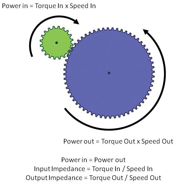
FIGURE 3. A gearbox transforms mechanical impedance from one combination of torque and speed to another, while losing as little power to friction as possible. The amount of transformation is determined by the number of teeth on each gear.
The situation is very similar to an RF transmitter designed for a load impedance of 50Ω but which can be connected to an antenna system presenting all sorts of different impedances. The electrical gearbox used here is known as an antenna tuner or transmatch.
One combination of voltage and current go in, and another combination of voltage and current come out, while heating up the matching unit with losses as little as possible. There are lots of different electronic components and circuits that can act as electrical gearboxes. Let’s meet a few of those.
Transformers
Resistive matching is not very useful if the goal is to deliver power efficiently, such as via the power grid. Instead, we use a transformer to change the high voltages and low currents of power distribution lines to the low voltages and higher currents in homes and businesses. Power is transferred as magnetic energy from the transformer’s primary to the secondary circuits through the transformer’s core. This is called a flux-coupled transformer.
Figure 4 shows the basic math for how a transformer converts impedances. Let’s say you have 115 VAC at the AC outlet and want 12 VAC for your project. Your step-down transformer would need a turns ratio of n = 115 / 12 = 9.6 from the secondary to the primary. If your project drew 1A of current, that 12Ω impedance would be transformed to a load of (12 V / 1 A) x n2 = 12 x 92.2 = 1106Ω to the AC line.
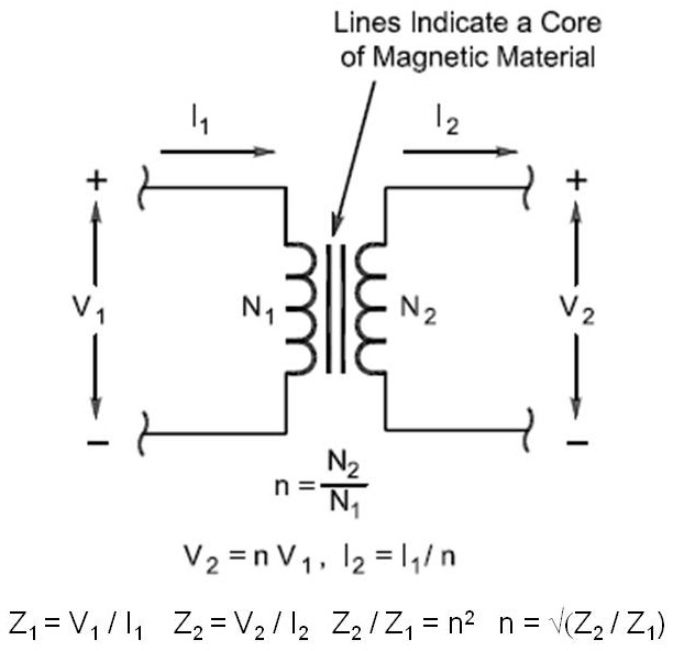
FIGURE 4. An electrical transformer transfers power with one combination of voltage and current (electrical impedance) through its core to another combination of voltage and current in the secondary circuit. The amount of transformation is determined by the ratio of turns on the transformer core's secondary winding to the number of turns on the primary winding.
You can find impedance matching transformers in many different types of electronic circuits. A very common use is to match the output of a transistor audio amplifier (which may have an output impedance of several hundred ohms of resistance) into the 4, 8, or 32Ω of speakers or headphones.
In ham radio, it’s not unusual for antenna systems to have impedances of 100Ω to 1,000Ω, so transformers are available with several selectable turns ratios to transform impedances by ratios of 2:1, 4:1, and 9:1. The result is an impedance that is close enough to 50Ω, so that either the transmitter is happy or only requires a little bit of impedance adjustment.
While power transformers for use at 50 Hz or 60 Hz have laminated steel or iron cores, transformers for RF use powdered iron or ferrite cores. If carefully made, RF transformers can be used over a wide bandwidth of 10:1, such as from 3 MHz to 30 MHz or from 150 MHz to 1,500 MHz. RF transformers are available for receiving and small-signal applications of a few milliwatts to high power transmitting units.
L-C Impedance Matching
An alternative to transformers are the L-C circuits or networks shown in Figure 5. These networks are composed entirely of reactive components (inductance and capacitance). The combinations of reactances transform voltages and currents at one side of the network to a different combination at the other by sharing stored energy as circulating voltages and currents. This electrical juggling act only works when the reactances have the right values, and that only occurs at one frequency since reactance depends on frequency.
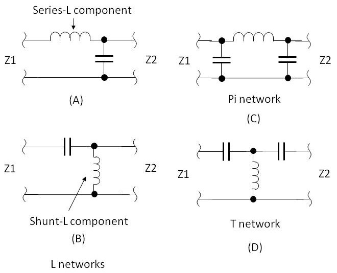
FIGURE 5. Four types of L-C impedance matching networks. Each type of network is named for the letter it resembles. A component in the signal path is called a series component. A component connected from the signal path to common or ground is called a shunt component. The circuit at A is a series-L shunt-C network, for example. The pi and T networks can each be viewed as back-to-back L networks as described in the text.
While four types of circuits are shown in the figure, there are many variations of each, and even other different circuits. Each of the networks is named for the letter which the arrangement of components resembles: L, pi (π), or T. Any of the Ls in the figure could be replaced by a C and vice versa, with the resulting circuit being able to transform different combinations of impedance.
The L network is very simple and works well for matching values of impedance that aren’t too different. (The more different Z1 and Z2 are, the higher the amplitudes of the circulating voltages and currents, and the higher the losses in the circuit components.) Each variation of the L network is capable of matching half of the possible combinations of input and output impedance. The remaining combinations can be matched by turning the network around. There is no dedicated input or output!
A calculator program (see the sidebar) determines values of L and C that create the impedance match. Out of the four L networks with one L and one C, two of the circuits will “work.” (For the other two circuits, no values of L and C are possible.) Of the two possible circuits, you can select the values of L and C that are most practical, the least expensive, or whatever is most suitable to your needs.
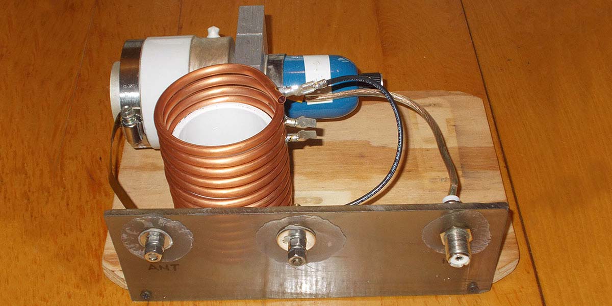
Figure 6 shows a high power L network that can handle more than a kilowatt of RF power at 3.55 MHz. Other L networks might handle only milliwatts of power.
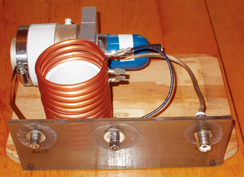
FIGURE 6. This L network is an example of the series-C shunt-L network in Figure 5B. Made from a heavy-duty coil and vacuum variable capacitor, it can easily handle 1 kW of RF.
The pi and T networks act like two L networks connected back-to-back. For example, if the series inductor of the pi network is replaced with a pair of inductors — each having half the original value — it is easy to see the input and output L networks. Similarly for the T network, the shunt inductor can be replaced with two double-value inductors in parallel, creating two back-to-back L networks. Why go to all that trouble when a simpler L network will do the job?
Remember that as the input and output impedances get farther apart, the circulating voltages and currents get larger. Another change is that the bandwidth over which the impedances can be considered matched shrinks. As the impedance ratio (also referred to as the network Q) increases, these two effects can make an L network impractical — particularly at transmitter power levels.
Pi and T networks are used to convert the impedances more gradually, putting less stress on the components. The resulting impedance match is made over a wider frequency range, too, requiring fewer adjustments as frequency changes.
Pi networks with series inductors are very common in HF (high frequency, 3-30 MHz) transmitter outputs because the series inductor acts as a filter to reduce higher frequency harmonics from the transmitter. An L-C network with inductors in the series signal path between input and output is called “low pass” because of the additional attenuation by the inductors at higher signal frequencies. This is useful in meeting FCC (Federal Communications Commission) specifications for transmitter output harmonics and other spurious emissions.
T networks are the most common type of circuit used for adjustable impedance matching units. These are high pass networks because of the series capacitance in the signal path. Even though these circuits don’t attenuate harmonics, the series capacitors make them less expensive to build and so they are popular in amateur equipment. Note that both the pi and T networks can be built with the opposite configuration of L and C, but those in the figure are the most common in use today for a variety of practical reasons.
Transmission Lines as Transformers
Transmission lines can be used to create reflections that cancel the unwanted reflections. Called synchronous transformers, the two best-known designs are shown in Figure 7.
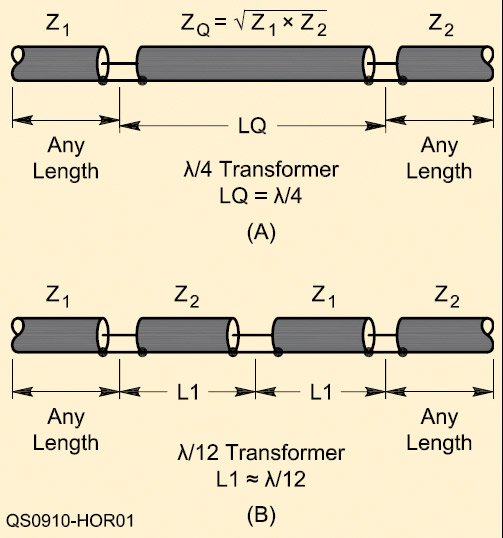
FIGURE 7. The quarter-wave transformer (or Q section) at A uses a quarter wavelength section of transmission line to match Z1 and Z2 by setting up reflections with the right phase to cancel all reflections from Z2. At B, two 12th wave sections match Z1 to Z2 without requiring a special section of transmission line.
The quarter-wave transformer (or Q section) works by inserting a length of transmission line between Z1 and Z2 that is one-quarter of a wavelength (λ) long at the frequency of the impedance match. The characteristic impedance of the matching section, ZQ, should be the geometric mean of Z1 and Z2 as shown in the figure.
For example, a one wavelength loop has a feed point impedance of around 120Ω. The geometric mean of 120Ω and 50Ω is 77.5Ω — quite close to the 75Ω impedance of RG-6, RG-59, or RG-11. There are many other types of coax with useful impedances, as well.
The Q section is found in many more places than just coaxial cable! If you wear glare-reducing coated glasses, the coating is a stack of transparent films. Each film is 1/4λ thick over a range of light wavelengths, and has a characteristic impedance such that the result is a set of canceling reflections created for a variety of wavelengths of visible light.
A similar trick is employed in the 12th wave section. Surplus CATV hardline is free or very cheap, but is usually 75Ω cable which would create a 1.5:1 SWR in a 50Ω system. By inserting two back-to-back 1/12th wavelength sections of the 75Ω and 50Ω cable as shown in the figure, reflections from the 75Ω cable are cancelled, making the system “look like” 50Ω — usually across an entire band of frequencies.
More Matching Material
We've barely scratched the surface of impedance matching techniques — a topic widely discussed in amateur radio. The ARRL has published many articles over the years but one of the best, "Another Look At Reflections," was written by Walt Maxwell W2DU. This multi-part article is available online at www.arrl.org/transmission-lines along with numerous other interesting and educational articles.
Are We Matched Yet?
I’ve presented four common techniques for impedance matching here: resistive, transformers, reactances, and transmission lines. You might recognize these in circuits you’ve seen on your workbench. Or, you might find one of these techniques to be just the thing you need to fix a pesky SWR problem or clean up some digital signals on a PCB. What’s important is to remember that once the frequencies of signals start exceeding a few hundred kHz, everything starts behaving like an RF signal — because it is! NV