(Above Photo Credit: J.L. Lee/NIST)
This November, in Versailles, France, representatives from 57 countries are expected to make history. They will vote to dramatically transform the international system that underpins global science and trade. This single action will finally realize scientists’ 150 year dream of a measurement system based entirely on fundamental properties of nature.
The International System of Units, informally known as the metric system — the way in which the world measures everything from coffee to the cosmos — will change in a way that is more profound than anything since its establishment following the French Revolution.
It will be a turning point for humanity.
Every day, scientists and engineers use measurements in design and research, but most of us give little thought to the basic definitions of our measurement system, and fewer still know that in the next year those definitions are in for some major changes. Take the volt, for example.
Readers of this magazine ought to know the definition of the volt, but I’ll bet that most don’t. I graduated with three engineering degrees and at the time, I could not have told you the definition of the volt. Last year, at my 50th college reunion, I gave a seminar in the EE Department on electrical metrology. Most of the EE professors and many students were present. I asked, “Who knows the definition of the volt?” … Silence.
One volt is defined as the difference in electric potential between two points on a conducting wire when an electric current of one ampere dissipates one watt of power between those points.
So, let’s talk about the volt. The volt is a derived unit which means that once the kilogram, meter, second, and ampere are defined, the equivalence of mechanical and electrical power dictates the definition of the volt. See the formal definition above.
The creation of the metric system in 1790 was the first time that scientists had the idea that measurement units should be connected with constants of nature. At the time, the Earth itself was seen as the best constant of nature. So, the second was defined as 1/86400 of a day, the meter was a best estimate of 10-7 of the distance from the equator to the north pole, and the kilogram was taken as 10-3 of the weight of a cubic meter of water.
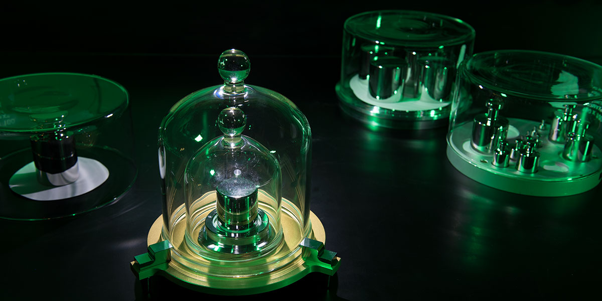
Since neither the surface of the Earth or a box of water make useful working standards, the formal definition of the meter became the distance between two scratches on a platinum iridium bar, and the kilogram became the mass of a cylinder of platinum-iridium. Both these artifact standards have been preserved for more than a century in a vault at the BIPM (Bureau International des Poids et Mesures) near Paris.
Beginning about 1900 with the development of quantum mechanics, it became clear that nature has constants that are more fundamental than the details of the Earth. With the invention of atomic clocks, the second was the first quantity to be redefined in terms of a fundamental constant and is now defined as the duration of 9 192 631 770 (ƒcs) oscillations of the Cesium atom.
In 1983, the invention of lasers allowed the speed of light to be defined as c = 299 792 458 m/s thus defining the meter.
The meter is the length of the path traveled by light in a vacuum during a time interval of 1/299 792 458 of a second.
The Josephson effect (V = hƒ/2e) has connected the volt to a known frequency ƒ and the constants h and e (e = electron charge and h = Planck’s constant). The Von Klitzing Effect has made possible a laboratory realization of the quantum resistance h/e2 = 25812.80757 ohms.
If we apply a Josephson voltage to the quantum resistance, Ohm’s Law gives the resulting current I = V/R = ƒ e / 2. Of the primary physical and electrical quantities, all but the kilogram now has a quantum realization. The kilogram has resisted redefinition for nearly five decades.
Even more concerning is that over the last 70 years, the artifact kilogram in Paris appears to have lost about 50 micrograms relative to six copies that — among themselves — are more stable. Only the kilogram is standing in the way of a redefinition of the metric system in terms of the fundamental constants e, h, c, and ƒces.
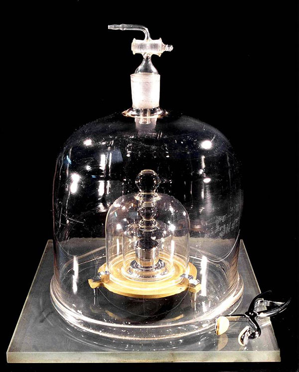
Figure 1. The golf ball sized cylinder of platinum-iridium that has defined the kilogram since 1905.
Think about it. At present, all our measurements of mass depend on a comparison to some other mass and ultimately to that block of platinum-iridium in Paris. How could we measure a mass in terms of fundamental constants? The first thought is Newton’s Second Law F = MA or M = F/A.
If we could apply a known force to an unknown mass and then m easure the acceleration, we could calculate the mass. The problem is that to be an improvement over the artifact kilogram, both A and F should be measured to better than about three parts in 108.
Acceleration can be measured with the required accuracy by counting fringes from a moving mirror in a laser interferometer. We can calculate a magnetic force between two current-carrying coils from knowledge of the currents and the detailed geometry of the coils. Unfortunately, uncertainty in the geometry leads to an uncertainty in the force that falls several orders of magnitude short of the required three parts in 108.
In 1980, Brian Kibble suggested a beautiful way to circumvent this problem. His apparatus is a balance scale. On one side is the unknown mass. On the other side is a coil that can move vertically in a magnetic field. The balance works in two modes: calibration mode and force mode.
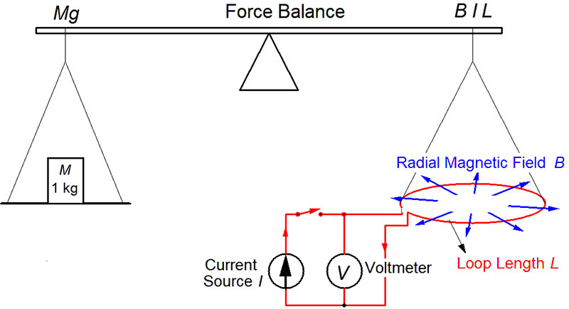
Figure 2. This apparatus compares electrical and mechanical power and is generally referred to as a watt balance (BL ≈ 50 Vs/m).
In calibration mode (switch open), the coil is moved vertically at constant speed S. From Faraday’s Law, this produces a voltage:
V = BLS
Since V and S can be measured with high accuracy, the product BL can be calculated BL = V / S — in effect calibrating the apparatus without the need for a detailed knowledge of the magnetic field or the coil geometry.
In force mode, a current I is applied to the coil to produce a force IBL to exactly balance the gravitational force Mg (g = acceleration of gravity) of the unknown mass. So, we have:
Mg = IBL or M = IBL / g
Assuming the product BL has not changed between the two modes, we can substitute the measurement of BL to get:
M = (I V) /( S g )
or
MgS = IV (Mechanical Power = Electrical Power)
V, S, I, and g can all be quantum-based measurements as described above. The equation above shows that this apparatus equates electrical and mechanical power, so it’s commonly called a Watt Balance. As a result from the Josephson equation for voltage of the volt, when we place a known mass on the balance, the experiment boils down to a measurement of Planck’s constant h in terms of the kilogram, meter, and second. Conversely, by defining the value of h together with already defined values of c and ƒcs, the kilogram becomes a quantum-based unit wholly derived from the definitions of e, h, c, and ƒcs.
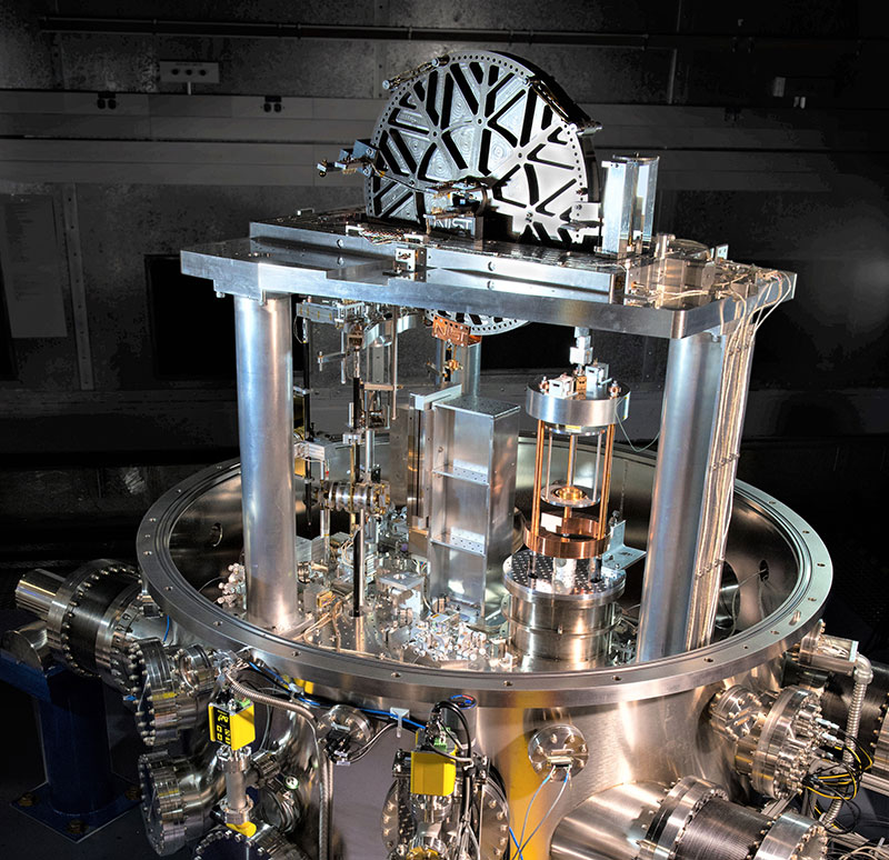
Figure 3. A watt balance constructed at NIST as part of the kilogram redefinition project. Note the bell jar at top that is lowered so that measurements are made in a vacuum to eliminate atmospheric buoyancy errors. (Photo Credit: J.L. Lee/NIST)
Needless to say, driving the uncertainty of this mass measurement below three parts in 108 is a daunting task that has been pursued at NIST and other national standards labs for almost four decades. After many redesigns and millions of dollars, the goal of three parts in 108 is clearly in sight. Independently designed experiments that are going on now around the world should soon confirm the viability of a quantum-based mass standard. If all goes as planned, the kilogram redefinition will occur in November of this year.
Looking at the big picture, over the last seven decades, the legacy artifact standards (meter, kilogram, second, and ampere) have been used to measure the constants of nature with ever greater accuracy; in each case, reaching an accuracy limited by the stability of those legacy standards. Going back to the original idea that our measurement system should be based on the constants of nature, the obvious path is to assign defined values to the electron charge e, Planck’s constant h, the speed of light c, and the cesium oscillation frequency ƒcs (or some similar quantum frequency).
With those four definitions soon to be formalized, all the quantities mass, distance, time, energy, power, voltage, current, and resistance will be measured in units derived from fundamental constants.
For metrologists, this is an earth-shaking change, but since the values of the fundamental constants will be chosen to align the old and new measurement systems, most of us will not notice the difference.
THE PROJECT
As a science project in do-it-yourself physics, it’s fun to imagine other ways to make a mass measurement by equating mechanical and electrical energy; something simple that might achieve 1% or better accuracy. My first thought was to use a DC motor to lift a mass M at a constant speed S.
Assuming no losses, we can equate the electrical power into the motor to the mechanical power of lifting M, so we have:
P = IV = MgS and M = IV
gS
I gave this a try, but unquantifiable losses in the motor and particularly the gear head made this method unacceptable.
From the point of view of universal elegance, the motor lifting experiment — as well as the watt balance experiment described above — fall short because both measurements must be performed in a measurable gravitational field. If we were traveling in a space ship to another solar system, these methods could not maintain a quantum-based mass standard along the way.
A Better Way
The gravity and gear head problems can be avoided if, instead of lifting the mass, we measure the energy required to spin a mass. Physics 101 tells us that the energy of a solid spinning cylinder is:
(π2 / 4) MD2 ƒ2
where M is the mass of the cylinder in kg, D is the diameter in meters, and ƒ is the rotational velocity in revolutions/second.
Now, suppose that we set the cylinder spinning with a motor and measure the electrical energy Ee = IVT required to spin the cylinder up to a rotational rate of ƒ in a time T. I and V are the current and voltage applied to the motor. Equating the electrical and mechanical energies, we have:
IVT = (π2 / 4) MD2 ƒ2 and solving for M M = 4IVT
π2D2ƒ2
This equation ignores electrical resistance loss and friction in the motor. As you will see in the circuit design that follows, we can measure and eliminate these losses.
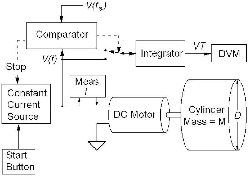
Figure 4. A concept diagram for measuring the mass of a spinning cylinder by equating mechanical and electrical energy.
Figure 4 shows a motor drive and measurement block diagram that when calibrated against standards of time, voltage, current, and length allows an accurate measurement of the product IVT and ƒ. Briefly, it works as follows:
We measure D with a digital caliper (our length standard). When the start button is pushed, a constant current is applied to the motor. As it spins up, ƒ is compared to a preset stop value ƒs. At the same time, the product VT is accumulated in an integrating amplifier. When ƒ = ƒs, the integration is shut off. I is measured with an ammeter. VT is measured with a voltmeter, and we have everything required to calculate M.
Figures 5 and 6 show a measurement circuit and its PCB (printed circuit board) that is designed to power the motor, plus make possible the accurate measurement I, VT, and ƒs by eliminating the effects of friction and resistance losses.
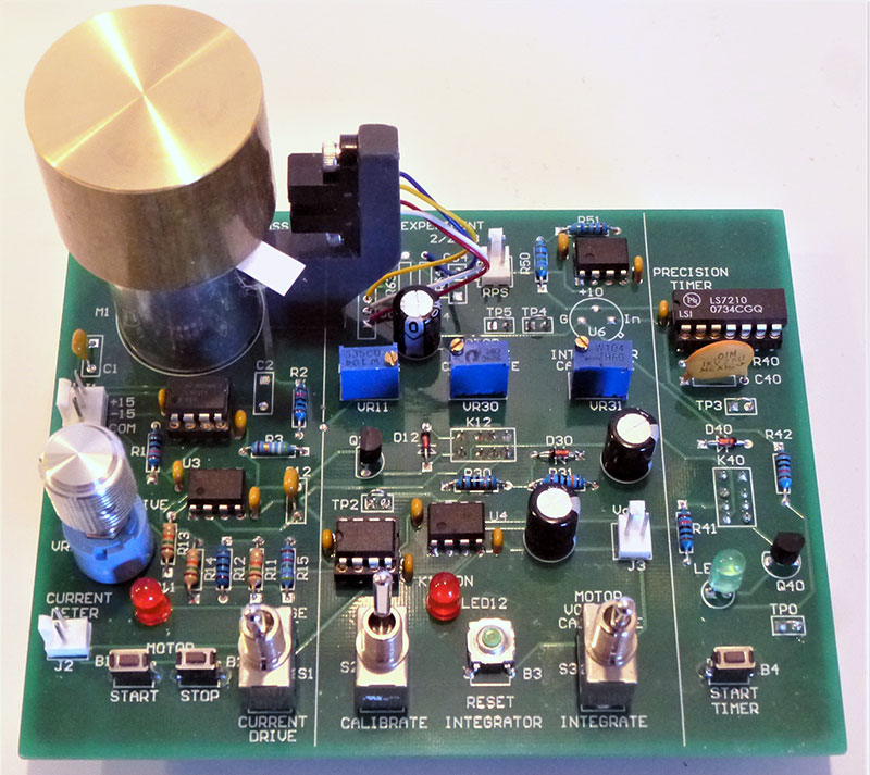
Figure 5. The PCB for the mass measurement experiment.

While Figure 6 looks complicated, it’s just the combination of four relatively simple circuits.
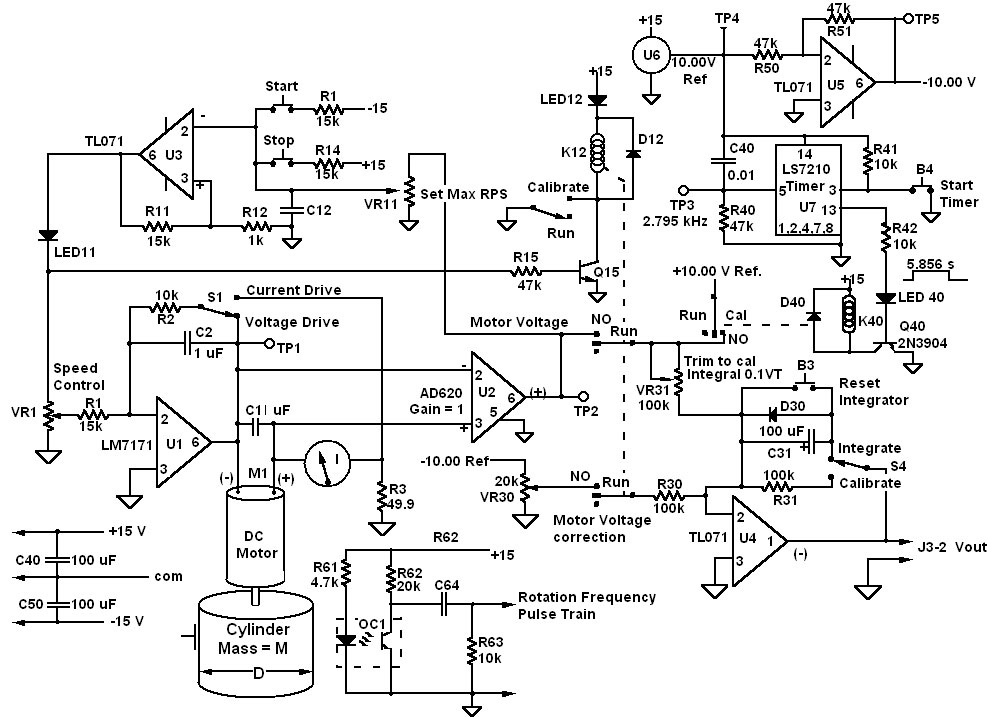
Figure 6. The schematic of the PCB in Figure 5
At the upper left, op-amp U3 uses positive feedback to implement a latching comparator. The start button latches the U3 output into positive saturation (13V), providing the control voltage for the motor and starting the voltage integration via relay K12. When the motor voltage rises to a value set by trimpot VR11, U3 will flip to negative saturation, turning off the motor and integration.
At the lower left, op-amp U1 (LM7171) provides a motor drive with ±100 mA capability. Depending on switch S1, the drive is constant voltage or constant current. Constant current is achieved by returning the motor current to ground through R3 and using the voltage across R3 as the feedback for U1.
A small paper tab on the rotating cylinder intersects an LED-detector pair to produce a pulse waveform at the rotation frequency. The frequency of this pulse waveform and thus the rotation rate can be measured with a frequency counter or oscilloscope.
At the upper right, U7 is a programmable timer that is used to calibrate the VT integrator U4. The LS7210 has an internal oscillator with a frequency set by C40 and R40; in this case, 2,795 Hz. The timer counts a specific number of oscillations set by five digital inputs at pins 9-13. Grounding only pin 13 sets the count at 16369, yielding a time delay of 5.856 s.
At the lower right is U4 — the VT integrator that is started and stopped by relay K12. Switch S4 selects resistive feedback through R31 for simply amplification, or capacitive feedback through C31 for integration. In integration mode, the U4 output ramps up at a rate proportional to the voltage input. Button B3 shorts the capacitor and resets the output to zero.
I designed the circuit using parts available in my shop, but if you buy it all, the total will be about $60 plus the PCB. The PCB and its layout files are available with the article downloads.
My motor was harvested from a defunct CD drive. I turned up the brass cylinder on my mini-lathe. Suitable disks in brass (~$20) or steel (~$5) are available from McMaster Carr. To run the experiment, you’ll also need a ±15V DC power supply, a digital voltmeter, and a frequency counter or oscilloscope.
CALIBRATION
The circuit of Figures 5 and 6 has five modes of operation: four calibration modes and one run mode. In mode 1, we’ll calibrate integrating amplifier U4 by applying a 10.00V reference voltage input for a precise time and then adjust the gain so that Vout equals exactly 0.1VT. The 10V reference voltage and Vout are both measured with our voltage standard: an Agilent 34420 six-digit voltmeter.
In mode 2, we calibrate the motor voltage by correcting out the component of motor voltage caused by the motor resistance. With 25 mA applied to the motor, we prevent the motor from spinning so that the motor voltage is I Rm where Rm is the resistance of the motor.
Trimpot VR30 is then adjusted to subtract the voltage I Rm from the input to the integrator. This ensures that the part of the motor voltage associated with resistive loss is excluded from the integrator output Vout.
In mode 3, we measure the motor voltage as a function of motor current when the motor is running at constant speed. Since there is no other load, all the motor current is used to overcome friction.
In Figure 7, we can see that the current required to overcome friction varies only from about 9 to 11 mA over the range from 0 to 7V So, in a spin-up from 0 to 7V, we can compensate for friction by subtracting 10.0 mA from the measured motor current.
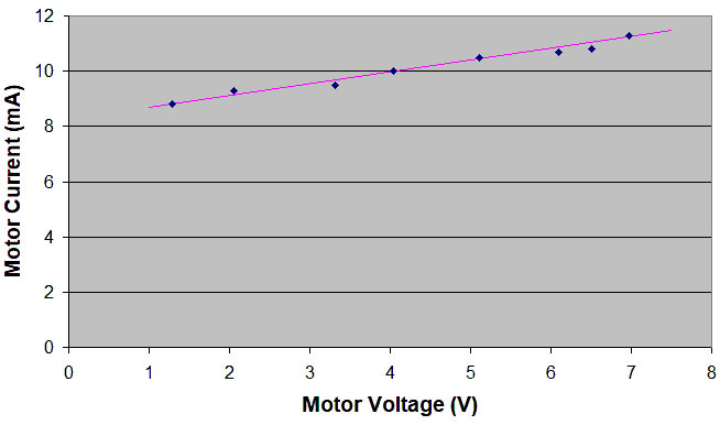
Figure 7. Motor current as a function of motor voltage.
In mode 4, we set the integration stop point to occur when the rotation rate ƒ is at a precise value. With 7V applied to the motor, adjust VR11 slowly CW until comparator U3 trips off. This sets the spin-up stop point at a known frequency ƒs, measured as described previously.
Mode 5 is the main measurement mode — what we’ve been getting ready for. Press the reset button to zero the integrator and the start button to start the spin-up and the VT integration. When the rotation rate ƒ reaches the set point ƒs, latch U3 will turn the motor and the integration off. The DVM will read the 0.1VT product — the last data point needed to calculate M.
Table 1 is a spreadsheet showing experimental data and the resulting mass calculation for a range of drive currents I and cut-off frequencies ƒs — all of which should produce the same result. The scatter of the results in Table 1 is a measure of the uncertainty of the mass determination.
| Cylinder Diameter (D) |
m |
0.0351 |
0.0351 |
0.0351 |
0.0351 |
0.0351 |
0.0351 |
| Applied Current |
A |
0.0209 |
0.026 |
0.0317 |
0.0317 |
0.0317 |
0.0399 |
| Friction Current |
A |
0.01 |
0.01 |
0.01 |
0.01 |
0.01 |
0.01 |
| Effective Current (I) |
A |
0.0109 |
0.016 |
0.0217 |
0.0217 |
0.0217 |
0.0299 |
| Measured VT |
V-s |
35.9 |
21 |
14.6 |
25.8 |
30.2 |
19 |
| Max RPS (F) |
Hz |
23.81 |
23.2 |
21.7 |
29.4 |
32.26 |
30.3 |
| Calc Mass |
Kg |
0.227 |
0.205 |
0.221 |
0.213 |
0.207 |
0.204 |
Table 1. Experimental Results.
The average of the five measurements shown is 0.213 Kg. I would expect it to be slightly high because I havn’t accounted for the mass of the rotating parts in the motor which add about 1% to the total moment of inertia. My kitchen scale gives the mass of the rotating cylinder as 0.210 Kg.
This little science project tries to give an inkling of the complexity of metrology research. It touches a multitude of areas in physics, electrical engineering, and metrology including energy, power, and moment of inertia calculations, op-amp circuit design, DC motors, error correction, and uncertainty analysis — a perfect combination for a physics or EE lab experiment.
The idea of a fundamental measurement of mass using a motor and a spinning flywheel was chosen because it’s doable with modest hardware and effort. I’m sure that NV readers will see a multitude of refinements and improvements — that is the stuff of metrology.
Refinement of the much more complex watt balance is a process that continues in multiple national standard laboratories around the world and is homing in on a mass uncertainty of three parts in 100,000,000 — roughly the weight of a fly’s wing relative to the kilogram. When that happens, the metric system will finally be defined in terms of the speed of light, the charge on an electron, the Planck constant, and the Cesium frequency. NV
Mass Experiment Parts List
| 4 |
TL071IP |
U3,U4,U5 |
Operational Amplifier |
| 1 |
AD620ANZ |
U2 |
Instrumentation Amplifier |
| 1 |
LM7171BIN |
U1 |
Op-Amp 100 mA |
| 2 |
AGN20012 |
K12,K40 |
12V DPDT Relay |
| 1 |
LT1460GCZ-10#PBF |
U6 |
10.00V Reference |
| 1 |
LS7210 |
U7 comes with PCB |
Programmable Timer |
| 3 |
|
LEDs 11,12,40 |
Red LED |
| 1 |
H21A1 |
OC1 |
Slotted Optical Switch |
| 2 |
2N3904 |
Q15,Q40 |
NPN Transistor |
| 4 |
EVQ-11A04M |
B1,B2,B3,B4 |
Tactile Switch |
| 3 |
1N914 |
D12,D30,D40 |
Diode |
| 1 |
MFR-25FBF52-49.9 |
R3 |
Resistor 49.9 ohms 1% |
| 2 |
MFR-25FBF52-1k |
R12,R64 |
Resistor 1K |
| 1 |
MFR-25FBF52-4.7k |
R61 |
Resistor 4.7K |
| 4 |
MFR-25FBF52-15k |
R1,R11,R13,R14 |
Resistor 15K |
| 3 |
MFR-25FBF52-10k |
R2,R41,R42 |
Resistor 10K 1% |
| 5 |
MFR-25FBF52-47k |
R15,R40,R50,R51,R62 |
Resistor 47K 1% |
| 2 |
MFR-25FBF52-100k |
R30,R31 |
Resistor 100K 1% |
| 1 |
Digi 496-2316ND |
C40 |
Capacitor 0.01 µF |
| 11 |
Digi 478-3192ND |
Bypass at op-amps |
Capacitor 0.1 µF |
| 3 |
Digi 399-4390ND |
C1,C12,C64 |
Capacitor 1 µF |
| 3 |
Digi 493-1548ND |
C31,C40,C50 |
Capacitor 100 µF |
| 1 |
Jameco 2217781 |
M1 |
DC Motor |
| 1 |
McMaster Carr 7786T12 |
Flywheel |
Flywheel, Steel |
| 1 |
PCB |
A limited supply is available in the NV webstore and comes with the LS7210* (U7). Gerber files are also available in the downloads. |
Downloads
What’s in the zip?
Gerber Files for PCB