Nowadays, there’s a ton of software kicking around to greatly simplify the design and construction of electronic circuits. Packages to capture schematics, perform simulations, lay out printed circuit boards, and so forth, abound. The trouble is, most non-professionals can’t justify the typically stiff expense of these, especially when not used on a daily, income-producing basis. But there is one software tool that most everyone can afford (in fact, you probably already own it) and it really does speed up the creation of many new circuits: the spreadsheet.
Like Edgar Allan Poe’s The Purloined Letter, the spreadsheet has been in full view for decades now and yet has remained virtually invisible to the average electronics enthusiast. Far from being only a financial tool, it can easily be coerced into performing a number of useful, repetitive, and complex operations that really take the tedium out of customizing circuits.
In a previous issue of Nuts & Volts, Peter Stark's article got the ball rolling by demonstrating how to apply spreadsheets to the digital world. The emphasis in this article is on analog design — an intimidating area to many since it often involves difficult or wearisome calculations. Not so anymore if you let the software help! You’ll learn how to get started and master the general methods, and as a side benefit, create some handy reference sheets you can put to use right away.
As mentioned, you may already have a spreadsheet program on your personal computer. But if not, don’t worry! The Resources sidebar shows some places where you can find inexpensive or even free spreadsheet programs. Most of these behave similarly, so the instructions given here (tested in Microsoft’s Excel program) will work with little or no change regardless of the package. If this all sounds intriguing, let’s dive in and see what’s possible.
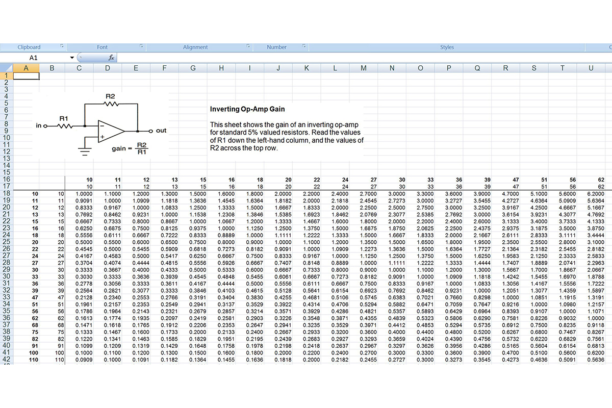
Suppose you need to amplify an audio signal by a certain fixed amount. The standard inverting op-amp configuration comes to mind, and indeed it’s easy to compute the gain of such a circuit: just divide the feedback resistance by the input resistance. But in this situation, we need to work backwards. We already know the desired gain and wish to learn which pair of resistors will create it.
You could try a bunch of different values on your pocket calculator, recomputing the gain for each pair until you hit the magic number. However, a slicker way is to simply let the spreadsheet program compute the ratio for every conceivable pair, and then read off the required combination. Best of all, if you print it out, you can punch it for a three-ring binder and have a ready reference for future work.
This is a simple example, but worth carrying out if for no other reason than that you can use it as a template for many different situations involving resistor pairs. Keep reading to learn how to implement it.
The Three Parts of an Electronics Sheet
To be most useful, an electronics spreadsheet should consist of three parts: a simple diagram or schematic showing to what situation the calculations apply, a brief verbal description of the circuit’s purpose, and the calculation table. If you include these three parts in every spreadsheet you create, then not only will you avoid the old “hmmm ... I forget what this is supposed to do” syndrome later on, but you can share it with other users and get your point across precisely.
So, the first step is to draw a simple schematic. For convenience, this is placed in the upper left-hand corner of the sheet. It could be drafted using nothing more than Windows Paint (which comes along for free with that operating system), the line-art tools that are part of Microsoft Office, or even a standalone drafting package that has an export option. Most spreadsheet programs let you embed a graphic directly. For example, in Excel, you go to the menu bar and select Insert>Picture>From File. File types like .gif, .jpg, .bmp, etc., are handled with ease.
Okay, so you’ve got the diagram in place now. Next to this, write up a brief description of what the sheet does and how to interpret the results. As mentioned above, this not only serves as a memory jog later on, but also makes the sheet more useful to others. In Microsoft Excel you could put this in a text box by clicking on that icon (it looks like a sheet of paper with a capital letter A on it), or you could simply enter the description in an empty cell, letting it spill over as needed.
Setting Up a Resistor Template
Now it’s time to work on the calculation table. For the inverting amplifier example, we’ll need to fill out a row and a column with the standard 5% values for resistors. You might object, thinking this to be a tedious task, but two things help here. First, remember that you need only do this once and can then use the sheet as a template for other resistor calculations later on. Also, there are a number of software tricks to greatly reduce the amount of typing required. Just follow these steps and see how fast it can be:
- Leave a couple blank rows at the top. Now starting at cell B3, enter the 23 standard 5% resistor values one after another down the column: 10, 11, 12, 13, 15, 16, 18, 20, 22, 24, 27, 30, 33, 36, 39, 47, 51, 56, 62, 68, 75, 82, and 91.
- The following entries come in decades. That is, 10 becomes 100, 11 becomes 110, eventually moving into the thousands, the tens-of-thousands, and so on. To automate this, with the cursor in the empty cell immediately below the last number you punched in (91), enter a formula that will create a result 10 times the value of the number in the top cell of that column (10).
Most modern spreadsheets let you do this with a combination of keyboard and mouse point-and-clicks. For example (depending what row you started with), the formula in this cell might appear as =B3*10. That’s what the formula looks like but, of course, it’ll be evaluated and displayed as 100, the next entry in the resistor sequence.
- Now simply replicate that cell over the remaining rows below. In Microsoft Excel, this is done by placing the cursor over the little square on the lower right-hand corner of the cell. The pointer will change to a cross. Now simply drag it down to row 141 and release the mouse button. All of the remaining values are magically created, from 10 Ω to 10 MΩ!
The replication process has copied the formula to successive cells, but since a relative reference is assumed, it’s revised to =B3*10, then to =B4*10, and so on. In some older spreadsheet programs, you may have to carry out this operation with a combination of copy and paste, but it’s still faster than typing everything in by hand since you can do dozens of numbers at once. While this may read long, in practice, you can create all 139 values in a minute or two and with very little keyboard work. (Of course, if you’re a zippy typist ...)
- Format the column any way you’d like. You could make the entries display as ordinary fixed-point numbers with commas, or in scientific notation, or whatever. It’s up to you, since the full precision values are maintained internally no matter how they appear on the screen.
So, you’ve got a column of standard values now, and these will refer to one of the resistors in our example. But with all those zeroes kicking around, it can be a little hard to read. So, in the first column (referenced as A on my system and deliberately left blank so far), type in the usual shorthand version for each number: 1K for 1,000, 330K for 330,000, and so on. These are just labels to make reading the table a little easier and don’t affect the calculations in any manner. You might want to format these with bold print to make them stand out a bit (see Figure 1).
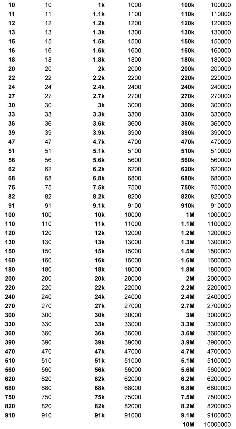
FIGURE 1. By exploiting a spreadsheet program's built-in Copy/Paste operations, you can create this array of resistor values with very little typing. Bold print labels for easy human interpretation are placed alongside the actual values used for computation. The numbers should actually be entered sequentially, although they're shown split into thirds here for better viewing.
Now we need to create a row of resistor values along the top. You could perform steps similar to what we’ve just completed, but there’s a faster way. Most spreadsheets have a variety of matrix operations built in, including one called Transpose. The purpose of this operation is to copy a row as a column and vice versa.
Consider the two columns so far as a matrix containing 139 rows and two columns. Invoke the Transpose function to create a new matrix from it containing two rows and 139 columns. In Excel, you can access this operation from the Paste Special menu. If the details hang you up somehow, be sure to check out the Help screens in your program.
Assuming everything’s gone well, you’ll rapidly end up with a copy of the first two columns, but arranged now as the top two rows. See Figure 2, and also notice how the schematic and text description referred to earlier appear at the top. Be sure to store your work in progress. You might also want to save this as a template, since it can be used for lots of different circuits involving two resistors.
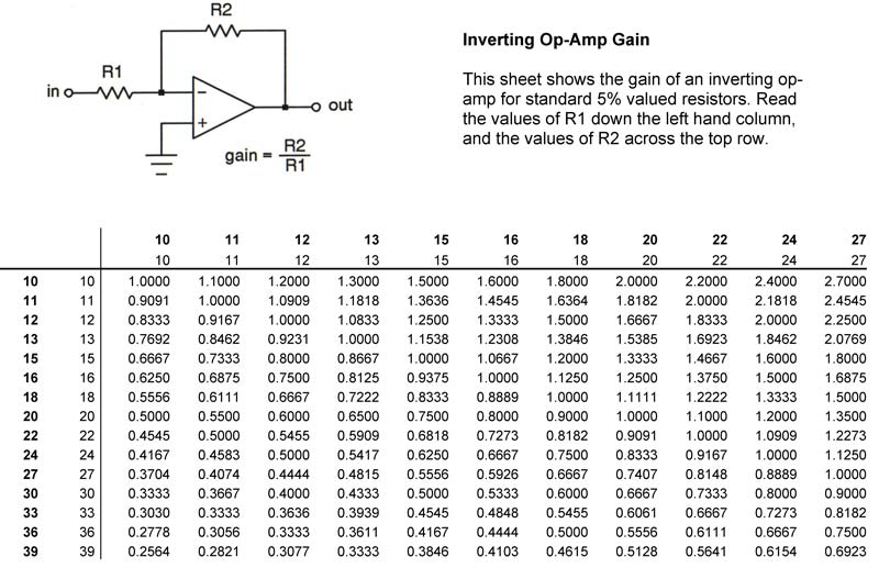
FIGURE 2. A portion of a basic design sheet. The entire table spans all values of 5% resistors from 10 Ω on up to 10 MΩ.
A Multitude of Calculations
Now comes the fun part — seeing the calculations fall into place! Plop the cursor down in the first empty cell at the intersection of R1 = 10 ohms and R2 = 10 ohms). Then enter the formula to calculate the ratio of these two. It should look something like this: =C$17/$B18 depending on which row and column you started with. With most spreadsheet programs, you can do a combination of keystrokes and mouse drag-and-drops to quickly enter this formula.
Pay close attention to the dollar signs in this expression. Normally, a spreadsheet defaults to a relative reference scheme (as it did when we entered the resistor values earlier). But in this case, we need to specify an absolute row or column, and that’s the purpose of the dollar sign flags. For example, C$17 says to reference the value which must be in row 17. On my system, this will be an R2 value. Then, we divide this by $B18, and this refers to a value which must lie in the B column. The B column contains the values of R1.
Finally, using drag-and-drop if your software permits it, or else a Copy/Paste operation, replicate this formula across the entire spreadsheet. Bang — in the blink of an eye, you’ll have the gain of an inverting op-amp for every possible pair of standard 5% value resistors! You should end up with a sheet like the one in Figure 2.
A More Complex Example
It’s all downhill from here. Not only do you have a template ideal for a variety of electronic design situations, but by following the steps detailed above, you’ve learned most of the tricks needed to massage a sheet into something useful. Here’s a more complicated example (in fact, a very tedious one to handle by hand with a pocket calculator) and yet it’ll only take you seconds to whip it up.
The problem is a common one: What will the output of a voltage divider be for various resistor strings, and for different input voltages? Figure 3 shows a portion of the resulting sheet. In this case, the computation depends on three quantities: R1, R2, and the applied voltage Vin. To make the sheet truly general-purpose, place the value of Vin in its own cell and label it. Position it in the upper left-hand corner of the table, so that it’s easy to spot.
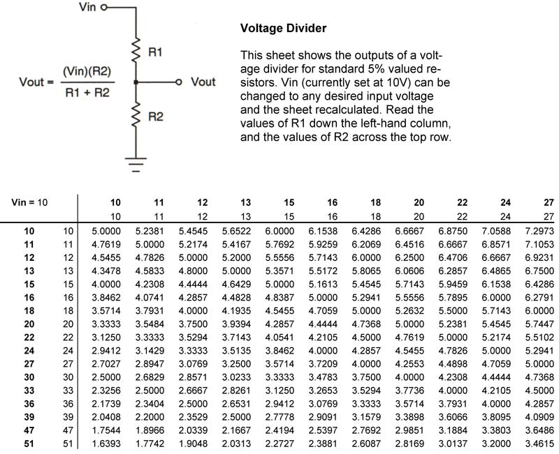
FIGURE 3. A slightly more complex design sheet. Again, only a portion is shown. Notice the parameter Vin, which appears in the upper left-hand corner of the table.
Now, have any calculations refer to this parameter instead of using an embedded constant. On my system, a typical entry looks like =$B$16*C$17/($B18+C$17). Again, watch the dollar signs. In this case, $B$16 refers to the absolute location of column 16 and row B, which contains the input voltage. When the sheet is filled out, you’ll see the output level for every combination of standard resistor values strung across 10V.
If you need to do it again, for 15V say, simply change that one single value in the upper left-hand corner and recalculate; the entire sheet is updated in a trice, and placing Vin in an easy-to-find locale makes it simple to experiment with many different voltages.
Much More Than DC Circuits
Creating spreadsheets for simple DC circuits is useful, and a great way to get started. However, there are many other unusual applications just waiting to be discovered. How about making a sheet to calculate the decibel equivalents of voltage ratios?
This is not only a handy reference to keep in your lab notebook, but also makes a great study aid should you wish to learn more about decibels and get an intuitive feel for what they mean. Figure 4 shows the layout.
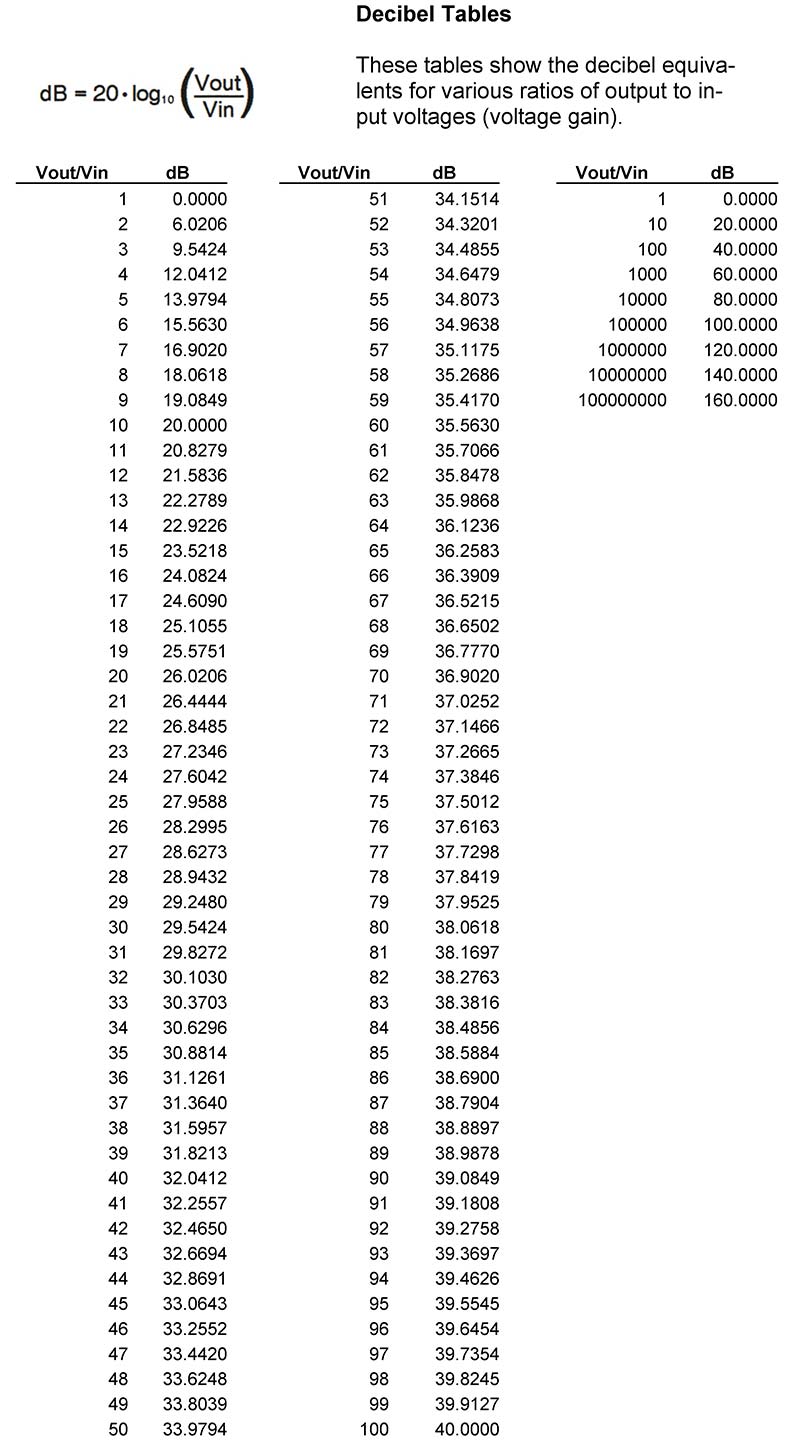
FIGURE 4. Decibel tables are great for home study.
To design this one, create a column of voltage ratios, starting at one and going as high as you want. For larger ratios, set out a second area where the jumps are bigger. Then simply copy in the standard formula =20*LOG10(A11). In this case, all references are relative and merely refer to the adjacent number in the A column, so there are no dollar signs. And LOG10 is nothing more than the base-10 logarithm function, part of every spreadsheet program’s bag of tricks.
Bring on the Capacitors
Now let’s up the ante a bit and see how to incorporate capacitance into our spreadsheet calculations. Here’s a practical example. Good quality audio circuits typically employ bandwidth limiting. This is to ensure that frequencies below and above the audio spectrum are rejected. The result is a circuit free of subsonic rumble or supersonic interference.
Figure 5 shows straightforward — yet reliable — circuits to handle both the low pass and high pass operations. Notice that one formula applies to both circuits, so you get double the bang for your buck here. That is, if the combination of R and C gives a cutoff frequency of 1,000 Hz, then in the low pass circuit, frequencies above this value are attenuated, and in the high pass version, frequencies below it are rolled off.
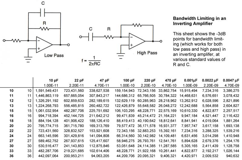
FIGURE 5. Here's a portion of a design table that makes designing reactive circuits — like filters — a snap. Actually, the resistors shown here are way too small for a practical circuit, so you'd want to use values further along in the list. Just scroll the table until you locate some reasonable numbers.
For this spreadsheet, you’ll need resistor values down the left-hand column, and capacitor values along the top row. The resistors we’ve already dealt with; you can simply use your template from before, keeping the column on the left but deleting the top row. Then punch in standard values for the capacitors. I used decade multiples of 2.2, 4.7, and 10, since these are the caps I usually have on hand. But feel free to employ any other intermediate ones you desire.
Since capacitance is typically quite small, there are lots of zeros and decimal places running around, which could make the table a bit hard on the eyes. So, as before, I created a row which gives the human equivalent as boldface labels (e.g., 100 pF), and immediately below this is the actul number to be used in the calculations (e.g., 1.00E-10).
If you’ve got your resistor and capacitor values punched in, then save this as a template, too. It’ll come in handy for all sorts of reactive circuits.
The formula you need for Figure 5 is =1/(2*PI()*$B18*C$17). The numbers and letters may vary, depending on what row and column you use to start your sheet. As usual, watch out for the dollar signs, since we want to grab resistor values from the column only, and capacitor values from the row only.
Here’s something new. The ubiquitous constant π (PI) shows up in the formula. Just about all spreadsheet programs have this built in, and by using it, you can get a good 15 decimal places of accuracy, much better than the lousy approximation 3.14 you used in junior high.
As an example of how quickly a problem can be dispatched with this sheet, imagine you wish to roll off the high end of an audio circuit at 100 kHz, say, to avoid spurious oscillations. Scrolling through the table you’ll instantly locate values of 75K and 22 pF for R and C, respectively. These will give a -3 dB point of 96,458 Hz, which is close enough. And you can look for other suitable combinations if you wish to raise or lower the resistor value to change the overall gain of the circuit. It’s a snap now!
Even Special Purpose ICs
Spreadsheets aren’t just for amplifiers. Use them to make working with more complex special-purpose integrated circuits easier. Just as an example, Figure 6 shows how to greatly simplify the frequency calculations of a function generator IC like the popular XR-2206.
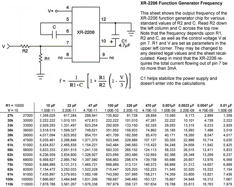
FIGURE 6. Spreadsheets can even simplify designing with special-purpose integrated circuits. Notice the two parameters R1 and V in the upper left-hand corner of the table. Only a portion of the sheet is shown here, and not all values at the extremes are practical for the XR-2206.
In this case, the output frequency (in Hertz) of the XR-2206 depends upon a pair of input resistors, a timing capacitor, and a control voltage. We’ll call these R1, R2, C, and V, respectively. Since we have four parameters here,and a spreadsheet is only a two-dimensional creature, what we’ll do is hold two of them fixed.
As Figure 6 shows, we start out with the basic resistor/capacitor template and then put R1 = 10000 and V = 10 in the upper left-hand corner to make them easy to spot. You can run the calculation and then if you’d like to see what happens when the control voltage drops to 5,V for example, merely substitute that number and recalculate.
The basic frequency formula for the XR-2206 is: =(1+($B$21/$B23)*(1-$B$22/3))/($B$21*C$22)
which is considerably more complex than any we’ve see so far. And yet, if you sort through it one step at a time, you’ll find there’s really nothing very new in it. For example, the $B$21 on my system refers to the absolute position of the cell in row 21 and column B; this is the resistor parameter R1. On the other hand, $B$22 is the control voltage constant, V.
The point here is most of us would never dream that a generic piece of software like a spreadsheet program could be applied so successfully to a special-purpose integrated circuit. And yet, assuming the chip manufacturer is courteous enough to provide reliable datasheets and formulas, we’ve seen that, in fact, you can really go to town.
And That’s Just the Start
Once I stumbled onto the notion of using spreadsheets for electronic design, I’ve been hooked ever since! I hope the examples presented here have piqued your interest and that you’ll consider creating and sharing your own spreadsheets for electronic design. The readers of Nuts & Volts comprise an active, generous community. Just imagine what kind of database we could come up with if everyone contributed a design sheet or two. NV
Downloads
Spreadsheet 2006-10 (analog design spreadsheets)