In this series of articles, we'll explore how to implement both analog and digital control systems. We will be using a PID (Proportional Integral Derivative) controller. With a PID controller, we can control thermal, electrical, chemical, and mechanical processes. The PID controller is found at the heart of many industrial control systems.
In this first of three installments, we will answer the “why” questions. We will also lay a foundation to better understand what a PID controller is. In subsequent installments, we will explore how to tune the PID controller and how to implement a digital PID using the ZILOG Encore! microprocessor.
The goal of this series is to introduce you to the world of control electronics. Concepts will be explained in a simple, intuitive fashion and useful, practical examples will be presented. The math will be kept to an absolute minimum. This is not to say that the math is not important. Quite the opposite — control systems may be modeled and analyzed mathematically. The mathematics is nothing short of amazing and I would encourage you to peruse it. There are hundreds of books that explain the theory and mathematics of control systems. These books will introduce you to powerful tools, such as Laplace transforms, root locus, and Bode plots. Again, this series of articles hardly scratches the surface. There is much more to be learned.
What Is PID Control?
The term PID is an acronym that stands for Proportional Integral Derivative. A PID controller is part of a feedback system. A PID system uses Proportional, Integral, and Derivative drive elements to control a process. Some of you already know what P, I, and D stand for. Don’t worry if you don’t; we will soon cover these terms with easy-to-understand examples.
Why Do I Need PID Control?
You need the PID because there are some things that are difficult to control using standard methods. Let me illustrate with an example. My first experience with control systems was a failure. My goal was to regulate the output of a power supply using a PIC microcontroller. The PIC read the output voltage with an AD converter and adjusted a PWM to regulate the output. The control strategy was very simple: If the voltage was below a set-point, turn on the PWM. If the measured voltage was above the set-point, then turn off the PWM. The PIC power supply almost worked. It did produce the DC output voltage that I wanted. Unfortunately, it also has a significant AC ripple riding on the DC signal.
The control strategy I just described is called on-off or bang-bang control. Many types of systems use this control strategy. Take the furnace in my house as an example. When the temperature is below the set-point, the furnace is on. When the temp is above the set-point, the furnace is off. Just like my power supply, the plot of temperature over time results in a sine wave.
For some types of control, this is acceptable; for others, it is not. You wouldn’t want this type of control for a servo motor — bad things would happen! Just imagine — the motor would be full power in one direction and, the next moment, full power in the other direction. You can see where the term bang-bang comes from. That servo won’t last long!
The PID controller takes control systems to the next level. It can provide a controlled — almost intelligent — drive for systems. We will now examine the individual components of the PID system. This step is necessary to understand the entire PID system. Please don’t skip this section; you must know how the individual components function to understand the whole system.
What Is Proportional?
This one is easy. The proportional component is simply gain. We can use an inverting op-amp, as shown in Figure 1.
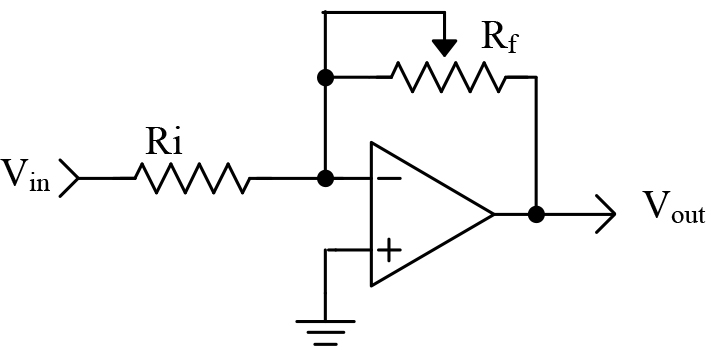
FIGURE 1.
In this op-amp circuit, the gain is set by the values of the resistors. We have the following mathematical relationship:
Vout = -Vin * Rf /Ri
What Is Integral?
Integral is shorthand for integration. You can think of this as accumulation (adding) of a quantity over time. For example, you are now integrating this information into your store of knowledge. Your store of knowledge has components of both time and knowledge. Obviously, we all started as babies with virtually no knowledge. Over time, we have integrated knowledge into our brains.
In our PID controller, we are integrating voltage as time progresses. A schematic of an integrator circuit is shown in Figure 2.
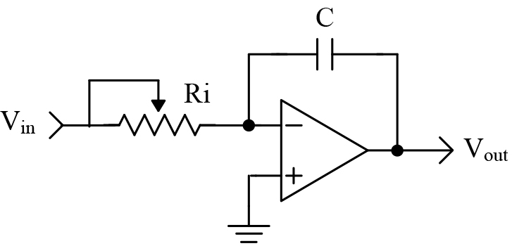
FIGURE 2.
The output voltage is described mathematically by the following equation:
Vout = -(1/RC) * (area under curve) + initial charge on capacitor
Area is a component of voltage and time. Let’s examine the operation of an ideal integrator. We can simplify the math by making the 1/RC term equal to 1 (i.e., let R=100 KΩ and C=10 µF). Figure 3 illustrates the input/output relationships of the integrator.
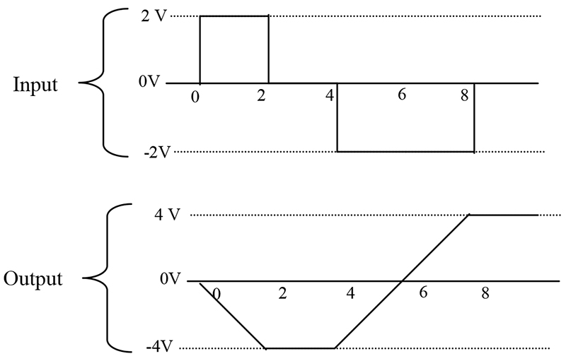
FIGURE 3.
From Time 0 to 2 seconds, have a 2 V square wave applied to the input of the integrator. The output of the integrator at the end of this time period is -4 V (remember the circuit is inverting). The integrator has accumulated a 2 V signal for 2 seconds. The area is equal to 4. From T2 to T4, there is no voltage applied to the integrator. The output is unchanged. In the remainder of this diagram, you can see that the integrator output changes polarity when the input signal changes polarity.
The previous discussion assumed an ideal integrator. Real capacitors will have some leakage and will tend to discharge themselves. Also, real op-amps may charge the capacitor with no input present. If the circuit is built as drawn, it will likely saturate after a few minutes of operation. To prevent this saturation, add a resistor in parallel to the capacitor. For our purposes, we are not concerned about the saturation. We will be using the integrator with other circuits to control the charge on the capacitor.
To better understand the integrator, let’s look at a typical application. Integrators are often found in high end audio amplifiers.
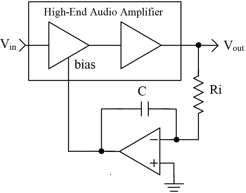
FIGURE 4.
In this application, they are called DC servos. A typical application is shown in Figure 5.
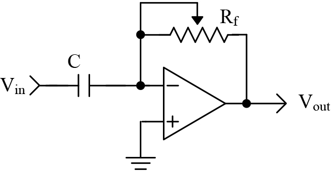
FIGURE 5.
The purpose of this circuit is to remove the unwanted DC voltage from the output of the audio amplifier. Any DC voltage seen on the output of the amplifier will tend to charge the integrator’s capacitor. The integrator then changes the bias of the audio amplifier to remove the DC component. The resistor and capacitor are selected so that the circuit will not respond to audio frequencies.
Also, recall that an AC waveform is symmetrical. The part above 0 tends to charge the capacitor, while the part below will discharge the capacitor. Therefore, when you integrate an AC waveform over a large amount of time, you get 0. Even a small DC voltage will charge the capacitor over a long period of time, thus rebiasing the amplifier.
What Is Derivative?
The derivative is a measurement of the rate of change. The ideal differentiator is shown in Figure 5. This circuit looks similar to the high pass filters you have seen in other schematics. Low frequencies are attenuated, while high frequencies are allowed to pass. The mathematics that describe the differentiator is:
Vout = -RC * (rate of change)
Rate of change is equivalent to measuring the slope of a line. Slope is a measure of the change in voltage divided by the change in time. In mathematical terms, this is referred to as a delta voltage over delta time or simply dv/dt. If we apply a ramp to the differentiator, we get a steady DC output voltage. Figure 6 illustrates the input/output relationship of a differentiator.
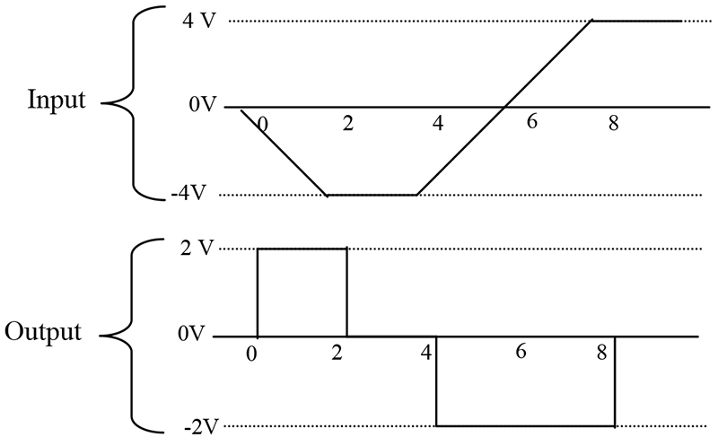
FIGURE 6.
To simplify the math, we will let RC=1. From time 0 to 2, the voltage changes -4 volts, while the time changes 2 seconds. The slope of this line is, therefore, -2. The output of the differentiator will be equal to 2 — remember the stage is inverting.
Servo Motor System
Now that we are familiar with the P, I, and D terms, let’s examine how they are combined to form a complete system. We will be using the PID controller to control a DC servo motor. I used a Hitec brand servo motor typically found in R/C model cars and airplanes. This servo is inexpensive and readily available. You can also purchase replacement gears — more of that in the next installment!
The servo mechanism consists of several components, as shown in Photo 1.
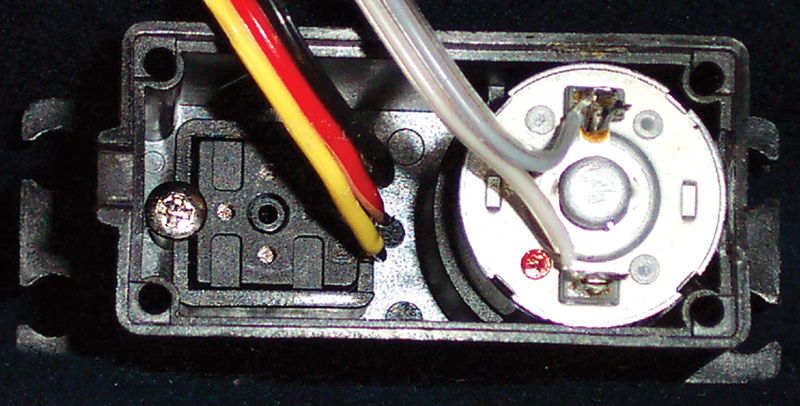
PHOTO 1.
We have a DC motor, a set of gears, and a variable resistor. The resistor is attached to the last gear. This variable resistor is used to determine the rotational position of the motor.
The servo was gutted. I only used the motor and the variable resistor, as shown in Photo 2.
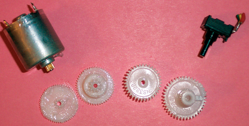
PHOTO 2.
PID Block Diagram
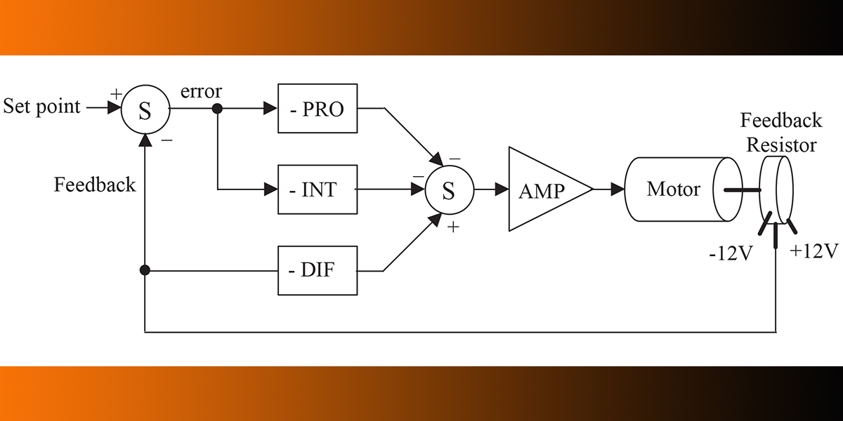
A block diagram showing the functional relationships of the PID controller is shown in Figure 7.
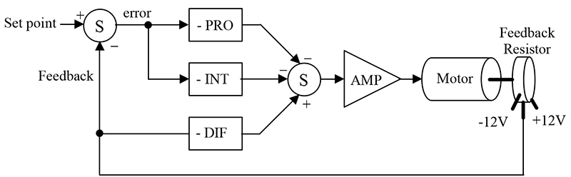
FIGURE 7.
The first thing to notice is that this is a parallel process. The P, I, and D terms are calculated independently and then added at the summer Σ. The input to this loop is the set-point — in this application, it can range from –12 to +12 VDC. The output is motor position. Position is measured by the resistor and feedback as a voltage between –12 to 12 VDC. We will now examine each of the PID terms independently to see how they are related. For this discussion, assume that the set-point is 0 VDC.
On the far left of Figure 7, we see a summing junction. The difference between the set-point and feedback is the error of the system. If the measured motor position is positive of where it should be, the error will be negative (i.e., a negative correction is required). Likewise, if the measured motor position is -1, the error will be positive 1 (i.e., a positive correction is required — remember set-point is 0 VDC).
The error is multiplied by the gain of the proportional block. Notice that the block diagram shows this as a negative gain. This was done so that the block diagram and the schematic (presented later) will be consistent with each other. The proportional amplifier output is sent to the second summing junction, where the sign is again inverted. The amplifier boots the signal’s current and drives the motor.
This chain gets to be quite long, so let’s summarize proportional operation in a few simple sentences:
- An error must be present!
- The system will try to correct the error by turning the motor in a direction that opposes the error.
- The intensity of the correction is determined by proportional gain. If there is no error, there is no proportional drive.
Moving on to integral — the integral is a device that charges a capacitor over a period of time. Recall the example of the audio amplifier. In that application, the integrator accumulated the DC output of the amplifier over time. It then rebiased the amplifier to eliminate the DC error. In the circuit in Figure 7, the integrator is performing the same task. It is integrating the error. It then provides a correction signal to the motor. We can summarize integral action in a few sentences:
- An error must be present!
- The integral section accumulates the error. A small error can become a large correction over a period of time.
- As the error is accumulated, the motor is forced to correct the error.
- Finally, the integrator will overshoot the set-point. It must produce an error opposite of the original in order to discharge the capacitor.
The final PID component is the derivative. Recall that the output of the differentiator was proportional to the slope of a wave. The same type of action is occurring in this circuit. When the motor starts to turn, the voltage measured by the resistor will be increasing or decreasing. If we have a voltage changing over a period of time, we have a ramp! The slope of this ramp changes with the speed of the motor. If the motor is going fast, the slope is high (i.e., voltage is changing fast for a given amount of time). Consequently, the output of the derivative stage will be high. The differentiator has the following attributes:
- The motor must be moving!
- The differentiator will have a high output voltage when the motor is moving fast and a low voltage when the motor is moving slow.
- This signal is applied in such a way as to slow down the motor.
- If the motor is not moving, the differentiator has 0 output voltage.
The connections for the differentiator are different than the proportional and integral sections. The differentiator receives its input directly from the resistor. It, therefore, measures only the speed at which the motor is moving. It does not care about the set-point. This is done to prevent large derivative drive signals when the set-point is changed. Again, the differentiator only responds to the speed of the motor.
Schematic
Figure 8 contains a simplified schematic of a servo motor PID control system.
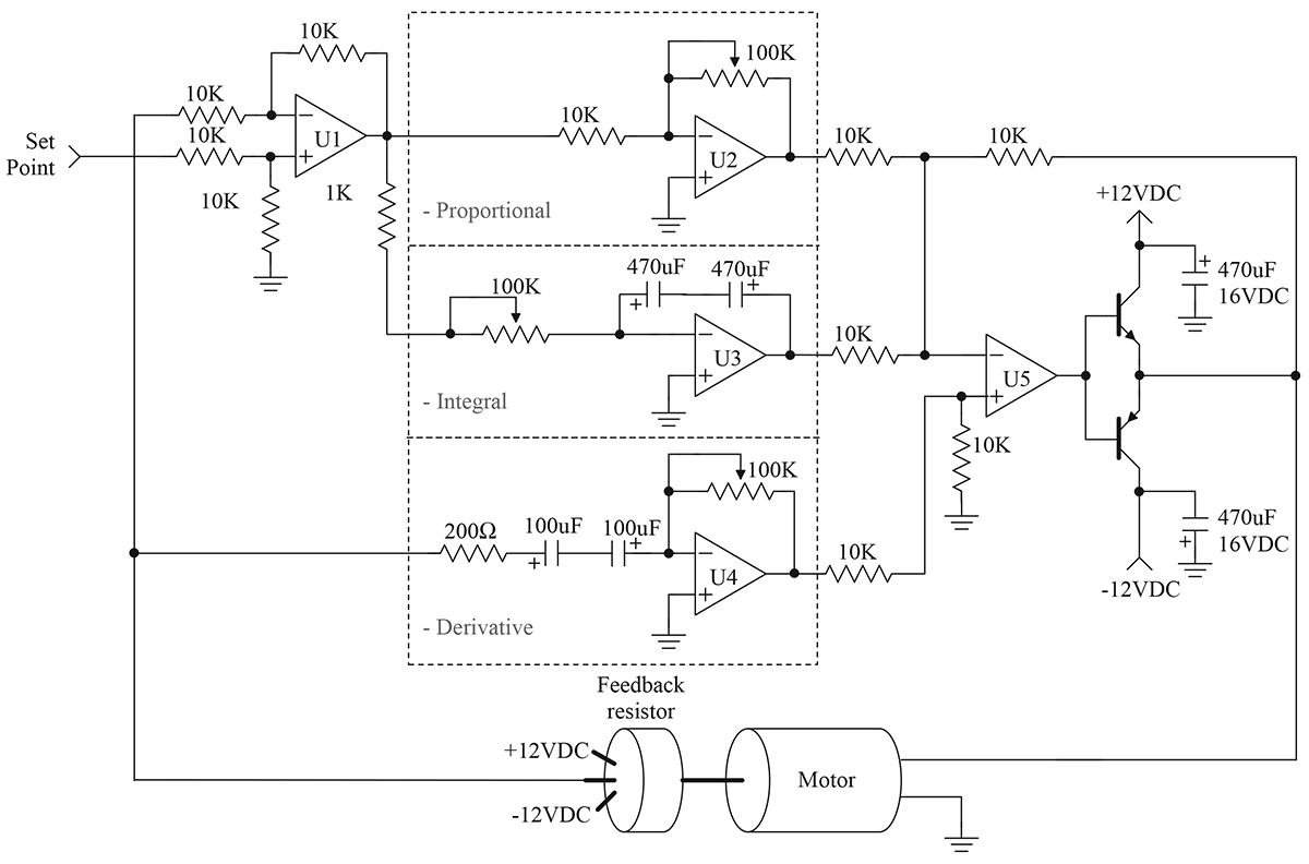
FIGURE 8.
This schematic is an adaptation of the PID controller presented by Professor Jacob in his book, Industrial Control Electronics. This type of system has the advantage of easy tuning. This circuit is also simple and easy to construct.
The schematic has the same physical layout as the block diagram. Op-amp U1 is used as the summing junction for the set-point and measured motor position. The individual P, I, and D functions are implemented by U2, U3, and U4, respectively. Finally, op-amp U5 sums the individual PID terms. The P and I terms are inverted, while the D term is not. Darlington transistors have been added to U5 to boost the current to a level sufficient to drive the motor.
The individual P, I, and D components appear just as they were presented earlier in this article. Each of the terms has a variable resistor to adjust its gains. The adjustment (tuning) of this circuit is the topic for the next installment.
Component selection for this circuit is not critical. The variable resistors should be multiturn for ease of adjustment. General-purpose op-amps may be used; however, U3 should be a FET input type. The FET design is better for the integrator, since it will not self-charge the integrator capacitor. I found a quad op-amp — such as the LF347N — to be ideal for this application. Large capacitors are required for the integrator and derivative circuits. The large values necessitate that electrolytic capacitors be used. The electrolytic capacitor may be operated as a non-polarized capacitor by placing two capacitors in series, as shown in the schematic.
Testing
Before we can test the PID circuit, we need to know more about the mechanical system. We need to know how it responds to a command and how the individual P, I, and D terms interact. You will have to be patient and wait for the next installment. In the meantime, go ahead and breadboard the circuit. You can use a function generator to verify the individual stages. See how the individual stages respond to sine, square, and triangle waveforms. Remember to use a low frequency — less than 10 Hz. This frequency is approximately the same as the servo motor system.
Stay tuned; next time, we will learn how to tune the PID controller. We will add additional circuitry to prevent a condition called integral wind-up. Also, keep a lookout for installment three, where we will implement the PID on a ZILOG Encore! microcontroller. NV
Downloads
PID Controller (Figure 8)