I’ve been using an oscilloscope for almost 50 years. It’s my go-to measurement instrument in every electronics project I work on, helping me debug and fine-tune hardware and software projects.
In this article, I’ll show how you can get started with a simple-to-use scope you probably already have. Best of all, it’s free! When you graduate from this simple scope, you can purchase a more powerful scope using the exact same user interface.
Full disclosure: I love scopes so much, 10 years ago, I joined Teledyne LeCroy — the third largest scope manufacturer in the world behind Tektronix and Keysight. However, I use the Digilent Analog Discovery 2 Scope (described in this article) in all my hobby activities and in the workshops I teach at Tinkermill — our hackerspace in Longmont, CO.
I think the free scope control software, Waveforms, is the simplest to use, most feature-rich pro-level software of any of the available options. Using a sound card as the hardware interface with Waveforms puts a simple — yet powerful — scope in your hands for free.
The Digilent Waveforms Software Interface
In June 2018, Digilent upgraded their software control tool (Waveforms) that runs their popular Analog Discovery 2 Scope. It now works with any sound card — either internal to the PC or connected through a USB port.
The very first step is to download and install the software. It will run on a PC, Mac, or Linux system. Download it from https://analogdiscovery.com/download by selecting your operating system.
Running this software on a PC will turn your sound card into an instant scope, capable of measuring audio range signals sampled at up to 100 kSamples/sec with a 16-bit analog-to-digital converter (ADC), with a built-in function generator based on a roughly 100 kS/sec digital-to-analog converter (DAC) — all controlled by an easy-to-use professional-level interface.
The free version of the software gives you all the extra features of a professional scope: time and voltage control; trigger options; spectrum analysis; datalogging; automatic measurements of figures of merit; serial data decode; and strip chart display. An example of the scope screen with just a few of these features is shown in Figure 1.
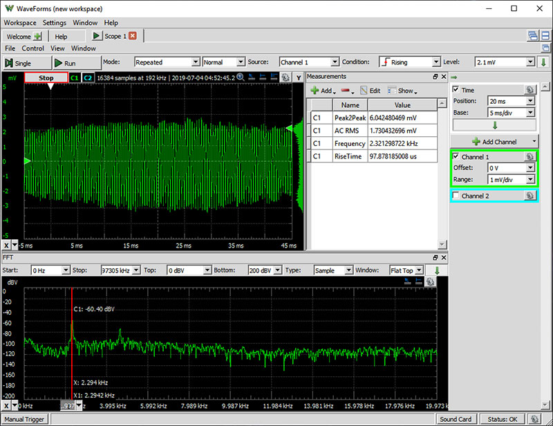
FIGURE 1. An example of a measurement of an incoming sound signal using the built-in microphone and sound card of my PC, displayed using Waveforms. The signal source was my short whistle, displayed in the time domain as a real time scope trace and in the frequency domain as a real time spectrum.
Here are just some of the functions you can perform with this software interface and a sound card:
- Measure voltage over time.
- Display the real time spectrum.
- Display the time evolution of the spectrum as a waterfall or spectrograph.
- Measure more than a dozen specific figures of merit of the waveform.
- Export the “voltage over time” data to a CSV file.
- Output a dozen different waveforms such as square, sine, triangle, and DC voltage at 100 kS/sec and up to 600 mV peak-to-peak values.
- Output a swept frequency signal or AM or FM modulated signal from 0.001 Hz to 50 kHz.
Turn Your Sound Card into a Scope
Using a sound card as a scope is not a new idea. After all, a sound card is nothing more than an ADC with a sampling rate of about 100,000 samples per second or 100 kS/s, with typically 16-bit resolution.
Even before you connect a sound card to the external world, you can explore the scope features using the built-in sound card in your computer, with its built-in microphone as input and speakers as output.
When you run Waveforms the first time, it will come up with a screen that says no hardware detected. After selecting OK, if you scroll to the bottom of the list on this screen, you’ll see your internal sound card listed. Select this, as shown in Figure 2.
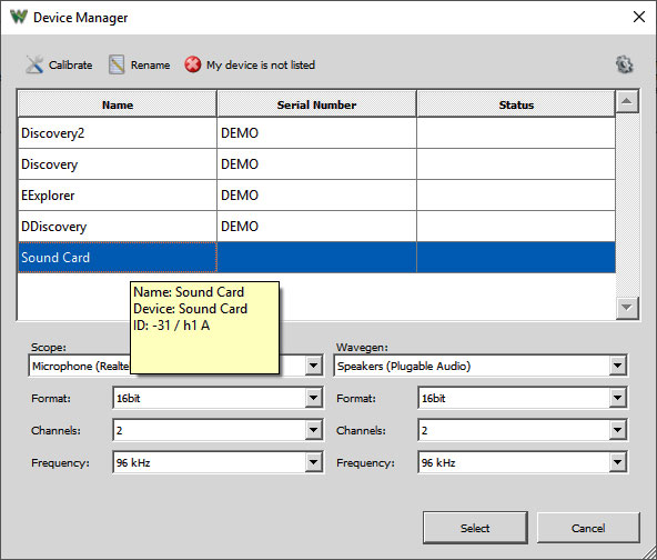
FIGURE 2. Select the sound card as the hardware option.
On the new screen, you’ll see the 12 different instrument icons on the left side. These are all available with the appropriate hardware front end. Using just the sound card, only seven of them are available.
To get started, click the scope instrument at the top of the list and the scope interface screen will pop up. Press the green run button right over the scope screen and you’ll see your first waveform.
Make a sound near your computer’s microphone input and you’ll see the voltage displayed on the screen from the internal ADC just using the default settings.
If you’re familiar with using scopes, this interface is very intuitive. You can display two input channels and adjust the vertical scale, the horizontal scale, and the trigger controls. The location of the menus for each of these are highlighted in Figure 3.
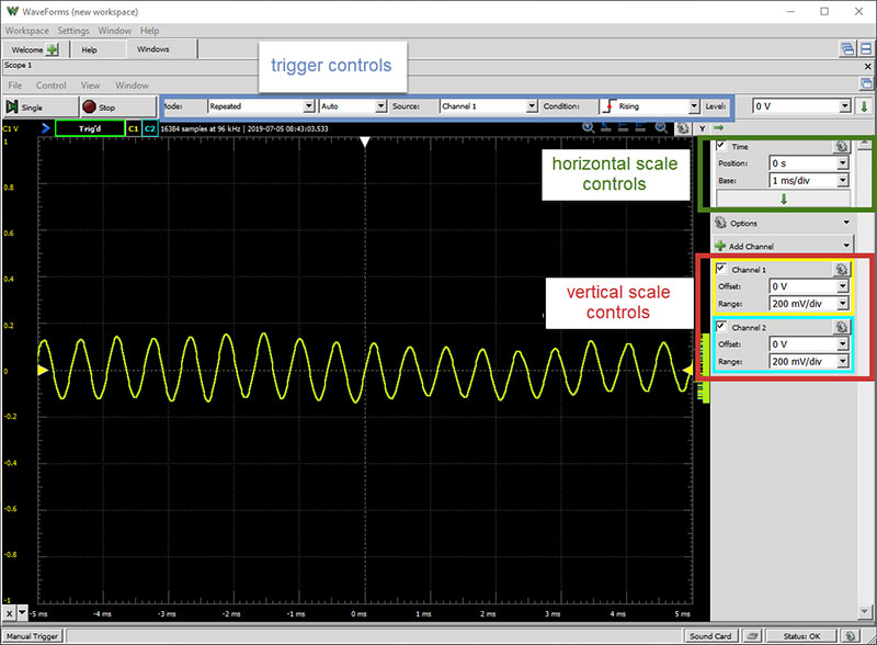
FIGURE 3. Location of basic scope controls, measuring an input from a whistle.
Operating a Scope for the First Time
An oscilloscope displays the measured voltage vs. time on the screen. While it looks like a continuous line, it’s actually composed of many individual measurements.
In the example above, the number of points in each acquisition (stored in the buffer and then plotted on the screen as one trace) is shown near the top of the display as 16,384 individual V(t) measurements.
In many scopes, changing the vertical and horizontal controls will also control the gain and sample rate of the internal ADC. This is NOT the case with the sound card scope.
Your sound card is taking data at a fixed rate; usually about 96 kS/sec and with a fixed full-scale voltage range at 16-bit resolution. It is fixed. The vertical and horizontal controls of the scope are just changing the display of these measurements.
We can control the vertical scale at which we plot the voltage values with the controls on the right-hand side. In this scope display, there are 10 vertical divisions. The scale for the voltage per division is adjusted with the Range control.
We adjust the vertical position of the 0V value on the screen with the Offset control. This is the additional voltage we are vertically shifting or offsetting the measured voltage on the screen.
When Offset is 100 mV, for example, the 0V level is shifted to the 100 mV position on the screen. If we wanted to center an input signal that was 3.3V then, we would want to shift the displayed voltage down 3.3V or use an offset of -3.3V. This would place 3.3V at the center of the screen.
The horizontal axis — divided into 10 divisions — is time. The time per division is set by the Base value. Where the time = 0 start is positioned on the screen is moved back in time with the Position control.
These are the two most important functions on EVERY scope. To get comfortable with these controls, spend some time playing with them using the background noise as the signal source.
Displaying Measurements on the Screen
The internal ADC in every scope will continuously measure the incoming voltage and send its data to the display buffer. How and when we display these voltage measurements on the screen is controlled by the Display mode and then the Trigger function.
The Waveforms tool has a rich selection of Display and Trigger features. In this short article, I’m going to touch on only a few of the basic ones.
At the top of the screen, “Mode:” has four options for how data is displayed in its pull-down menu.
The Repeated option is how a scope usually displays the data. Each acquisition is plotted as the voltage(t). After each acquisition is triggered, the old data is erased and the new buffer is plotted. It happens so fast that it looks like all the data suddenly appears on the screen at one time. This mode is available only when the time base is 50 msec per division or shorter, which means the last 500 msec of data is displayed.
When the time base is 100 msec/div or longer (in other words, when you want to display one seconds’ worth of data or longer), the scope switches to one of two Display modes.
The Shift mode turns the scope into a strip chart recorder. The data is measured and streamed to the display putting each new measurement on the right-most position and shifting all the old data to the left. This looks like what you see in an EKG, for example, with a strip of paper rolling out.
The Screen mode does the opposite. Each buffer acquisition is painted on the screen with the most recent data on the left, over-writing in real time the previous set of data as it comes in. This makes it look like the heart rate monitors you see in hospitals.
For all the fast signals we measure that will use a time base of 50 msec/div or shorter, only the Repeated mode is available. This is how we are used to seeing a scope.
The Trigger mode determines when the buffer of data gets displayed on the screen. This is probably the most confusing control and yet the most important function to master for any scope.
Triggering the Scope
The ADC is taking data all the time and placing it in a first in, first out (FIFO) buffer. Think of it as a train with 16,384 (the number of measurements in one acquisition) little box cars all going around a closed circular track.
At the train station, each consecutive ADC measurement is placed in an adjacent car as it goes by. As the first car comes back to the station again, its previous measurement is replaced with the new measurement.
In Normal trigger mode, none of this new data gets displayed to the screen unless the current measurement is above a trigger level and the signal is either rising or falling. Time (t = 0) is defined by when the measured voltage exceeds the threshold. Then, all the data that is acquired for t > 0 is displayed.
If you happen to have the position of t = 0 on at the middle of the screen, you also get to see the data that was in the train before the trigger signal was reached. This is how the scope is able to “look back in time” from before the trigger threshold was reached.
To illustrate this, I set the trigger to 300 mV in Normal trigger mode and added a horizontal cursor at 300 mV, so you can more easily see the threshold level of the trigger. When the input signal level exceeded 300 mV, the past measurements and future measurements that could fit on the screen were displayed. That’s what we see in Figure 4.
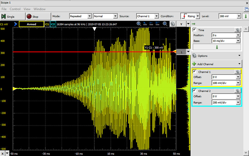
FIGURE 4. In Normal trigger mode, t = 0 is defined as when the voltage exceeds the threshold value and the data is displayed.
In Normal trigger mode, if the trigger voltage is never reached, the data is never displayed on the screen. All you see is the previous trace from the last trigger. It looks like the scope is dead. Data is only displayed if the incoming voltage reaches above the set threshold.
Using Auto trigger mode is exactly the same as Normal trigger mode, except that if no valid trigger signal is received for some period of time (like two seconds), the scope will trigger anyway, showing whatever is in its acquisition buffer. This way, you get to see triggered signals (if there are any), but if there aren’t or you adjusted the trigger incorrectly, you can still see what the ADC is measuring.
Once the scope waits two seconds after not receiving a valid trigger, it will continue triggering as though it were getting a continuous trigger signal. This is the same operation as None trigger mode. The scope just displays the most recent buffer of measurements as though it was getting a valid trigger signal after each acquisition.
There is another mode which is controlled by the buttons to the right of the Mode. This will enable a single-shot display. The advantage is that this will hold the last triggered measurement and not overwrite it if another trigger signal comes in. This makes it easy to see a short-lived transient event.
Practical Habits
The default settings of the Waveforms software are a good place to start every measurement. The scope should be set for Auto trigger mode. Adjust the time base to 1 msec/div and offset to 0. Adjust the vertical scale to 200 mV/div and 0 offset.
You should see measurements displayed. At this point, it’s important to just play. Adjust the scales and trigger and get a feel for how you can adjust the screen to display the same data in a way that makes the measurement most clear. For me, I like to see nice whole numbers as the vertical and horizontal values displayed. This means adjusting the offsets to get whole numbers as the scale values.
Try clapping your hands, snapping your finger, whistling, talking, or playing the radio as inputs and find the best settings to display these signals.
Using the free Waveforms tool and the built-in sound card, you can become a master at using a scope interface. Then, you’re ready to move on to using the sound card to measure external signals.
Reverse Engineering a Typical Sound Card’s Performance
The limitations of using a sound card scope are due to the performance of your sound card. There is a limit to the lowest frequency and highest frequency that can be measured and to the highest voltage and lowest voltage.
These values are typically not specified anywhere in a sound card’s documentation. The only way to get this important information is by reverse engineering them from actual measurements using a reference source. I used my Digilent Analog Discovery 2 Scope as the reference signal generator. You can also use the digital signals from an Arduino to get a simple calibration.
Whenever you connect an external signal to your sound card, you run the risk of possibly applying too large a transient voltage and blowing out the front end of the sound card. While all sound card inputs are AC coupled and generally ESD (electrostatic discharge) protected, there is always a risk of damaging it. You do not want to destroy your PC’s built-in sound card!
To reduce this risk, I strongly recommend when you want to connect an external signal from one of your projects, do not use your internal sound card. Instead, purchase a low cost external USB sound card.
For example, the Sabrent (https://www.sabrent.com/product/AU-MMSA/usb-external-stereo-3d-sound-adapter-black/#description) low cost ($8) USB sound card has an internal 16-bit ADC that can sample up to 196 kS/sec, but has a limited input frequency range from about 100 Hz to 20 kHz. The Waveforms software tool can drive this USB sound card.
To connect the real world to a sound card, I used a common audio stereo cable plugged into the sound card and a microphone socket. I purchased 10 of these sockets for $11 on Amazon. I wired three solid core hookup jumpers to the PCB (printed circuit board) mount socket. This end is shown in Figure 5.
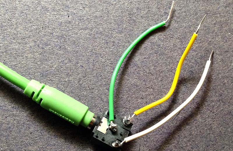
FIGURE 5. Close-up of the stereo audio socket with the cable to the sound card and the wires to my DUT.
To test the input measurement range of the Sabrent USB sound card, I created a sine wave signal source using my Discovery 2 Scope with built-in function generator. The amplitude was constant from DC to 10 MHz. I measured this sine wave signal with the Sabrent sound card using the Waveforms interface. Figure 6 is an example of the measured sine wave set for 1 kHz.
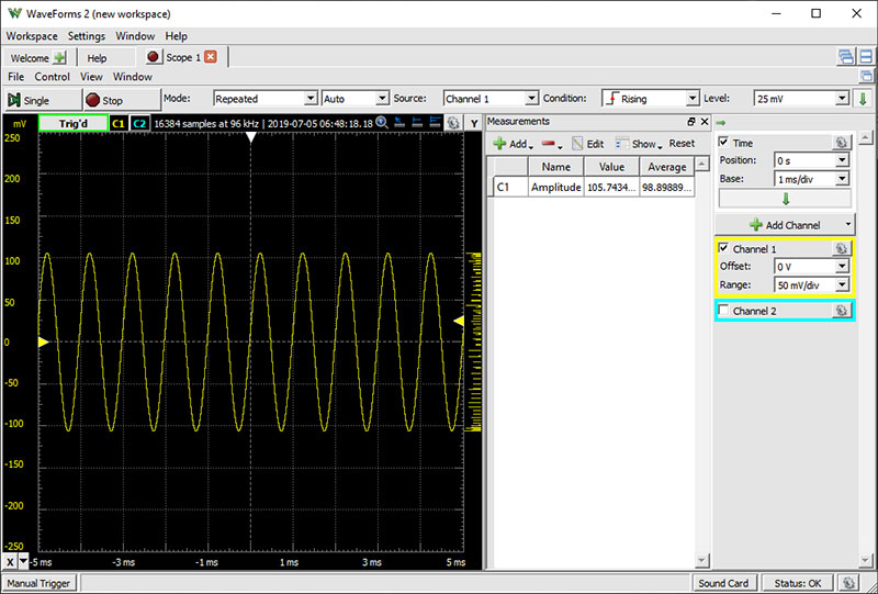
FIGURE 6. Measured input to the sound card with a 1 kHz sine wave as the source.
I measured the sine wave amplitude displayed from the sound card at different frequencies. Figure 7 shows the ratio of the measured sine wave amplitude at different frequencies, normalized to the amplitude that got through the passband region.
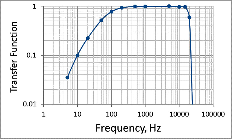
FIGURE 7. Response of the ADC built into the Sabrent sound card to sine waves.
When plotted on a log-log scale, this sort of plot is called a Bode Plot. It’s the transfer function of the relative voltage measured by the sound card.
From the Bode Plot, we see that the lowest frequency at which we can still measure about 70% of the input voltage — the -3 dB point — is about 90 Hz. The highest frequency for which the displayed voltage is within -3 dB of the passband voltage is about 20 kHz.
The low frequency behavior matches what we would expect for a single pole RC high pass filter with a pole frequency of 90 Hz. The ADC input is capacitively coupled to block DC voltages, and there is some resistance on the other side across the input to the ADC.
If we drive the input to the ADC with a square wave, we’ll see the peak get through, but then drop off with a time constant equal to:
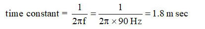
The transient response of the sound card scope to a square wave will be pulses on each edge with a 1.8 msec decay time. This is exactly what I measured. Figure 8 shows the 100 Hz square wave input to the ADC and the resulting measured voltage by the sound card. The 4V peak-to-peak edge comes through, with the DC level dropping off with a time constant consistent with 1.8 msec.
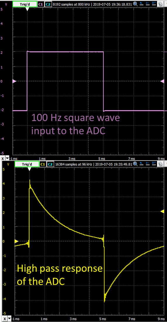
FIGURE 8. Top: The input voltage to the ADC. Bottom: The displayed ADC response being the high pass filtered square wave with a roughly 1.8 msec time constant.
What this behavior illustrates is the limitations of any sound card scope. Because of the poor low frequency response, we can only see the edges of signals. This makes it not very useful to look at slowly varying analog signals, but well suited to measure audio signals above 100 Hz or the pattern of digital signals such as the outputs of digital pins on an Arduino.
The maximum input voltage (as measured by the Discovery 2 Scope) I could apply before the sound card scope displayed-voltage saturated was about ±300 mV.
If this is the voltage range of the 16-bit ADC, the smallest voltage we can measure (in one bit-level) is 600 mV/65,535 = 0.009 mV or 9 µV. This is a very sensitive ADC.
However, this low a value for the maximum input range the ADC can measure is a significant limitation. Applying a larger input voltage above ± 0.3V would saturate the ADC, and more importantly, run the risk of damaging it. To measure 5V signals that I might find on an Arduino, I need to add an attenuating interface circuit between the voltage to measure and the input to the sound card microphone channel.
Interfacing the Sound Card to the Real World
The maximum tip voltage I can apply is ±0.3V. I need to add a voltage divider to the front of the sound card to drop the tip voltage from 5V to lower than 0.3V. This is a voltage divider of 0.3V out with 5V in, or a ratio of (at most) 0.3V/5V = 0.06. I can build this with a simple resistor voltage divider. I selected resistor values of 10K ohms and 330 ohms. Their voltage divider ratio is 330/10,330 = 0.03, which is below our requirement of 0.06. These values are commonly found in many kits. The exact values are not critical, as long as the voltage divider ratio is below 0.06. It would make the input impedance to the sound card 10K ohms, which is a reasonable value to not load down a circuit.
The equivalent circuit and what I set up is shown in Figure 9. With this circuit, a 5V signal at the tip will create a 5V x 0.03 = 0.15V signal into the mic input. This is below any voltage to worry about with the ADC.
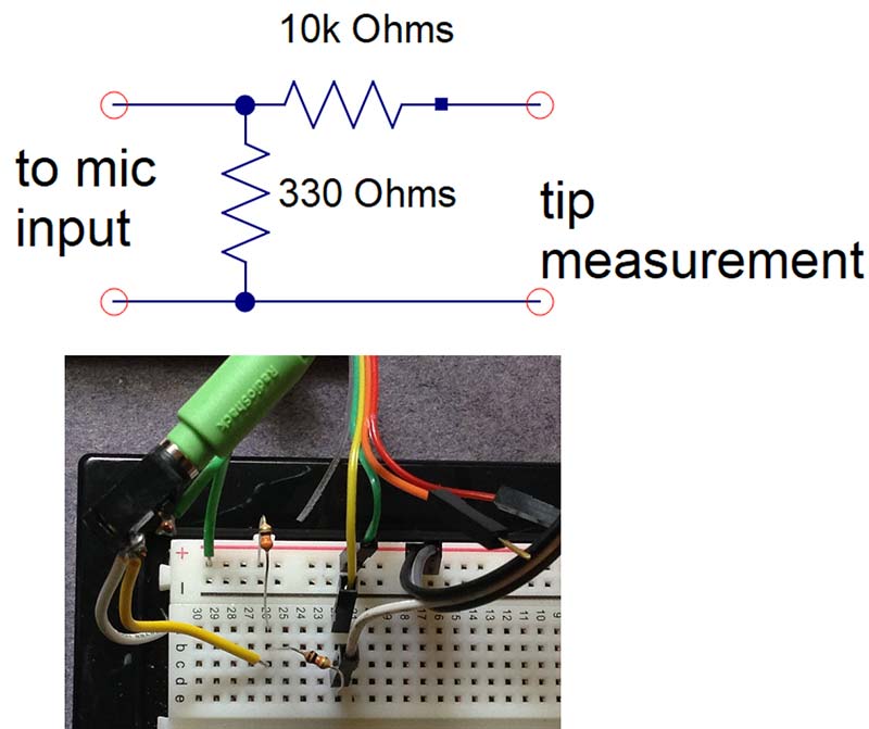
FIGURE 9. Top is the voltage divider circuit and bottom is the actual solderless breadboard version.
And, with the smallest voltage of 9 µV for each digitizing level at the mic input, this would correspond to a smallest tip voltage I can measure of 9 µV/0.03 = 0.3 mV — plenty of sensitivity.
Calibrating the Sound Card Scope
The final step is to adjust the channel attenuation factor to make the displayed voltage on the scope equal to the actual tip voltage.
The displayed voltage from the sound card’s ADC is NOT a calibrated measure of the input voltage to the ADC. It’s just a value generated by the Waveforms software based on the ADC count value and an assumption about the ADC range and resolution. This — plus the resistor network — means the displayed voltage and the actual tip voltage will not likely be the same.
Built into each channel of Waveforms is a calibration factor — labeled as Attenuation — that will allow us to rescale the displayed screen.
This Attenuation term is a little confusing. It’s really designed to adjust the displayed screen voltage to equal the tip voltage when using an attenuating probe like the commonly used 10x passive probe.
A 10x probe is not really a 10x probe. It’s a 1/10th probe. The voltage displayed on the scope screen is 1/10th the actual voltage at the tip of the probe attached to the DUT (device under test). Yet, we call this a 10x probe.
If we were using the Analog Discovery Scope and had a 10x probe connected to the scope, and we wanted the scope to display the actual voltage at the tip, we would use an attenuation setting of 10x in the channel setting. The voltage displayed on the screen would then be the tip voltage.
To find the correct attenuation value to use, we apply a known signal to the tip and observe the voltage value displayed on the screen with an attenuation value of 1x. We then calculate the attenuation value to type in as:
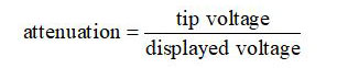
This is the value we type in the Attenuation box in the channel setup, as shown in Figure 10.
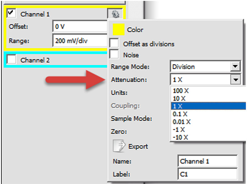
FIGURE 10. Under the gear symbol for the channel, select the Attenuation box and type in the value here.
I used my Discovery Scope as a function generator and provided a 2V peak-to-peak sine wave at 1 kHz. The maximum voltage range of the function generator is ±2V.
I measured the actual tip voltage as 2.00V peak-to-peak. I then measured the voltage displayed on the screen as 0.212V peak-to-peak. This combines the factor of 0.03 attenuation in the resistor divider circuit and the ADC calibration. The Attenuation value is:
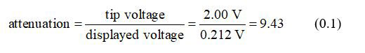
This is the value I used in the Attenuation factor term. Using this term, I now measure a peak-to-peak voltage of 2.00V on the sound card scope screen.
An alternative signal source could be the 5V digital signal from an Arduino pin. Adjust the Attenuation factor so that when a 5V signal is the input, you see a 5V peak-to-peak edge displayed on the scope. Just use a long enough off time to see the signal decay to 0V.
Measuring Arduino Signals
Due to the high pass filter built into the ADC, the sound card scope will mostly see the edges of digital signals. This makes it ideal to see the frequency and duty cycle of signals, such as from pulse width modulated (PWM) signals.
I wrote a simple Arduino sketch to drive a 50/255 = 19.6% duty cycle PWM signal on pin 10 using digitalWrite(10,50). Figure 11 shows the signal at the pin, as measured by the Analog Discovery Scope hardware and the signal measured by the sound card scope.
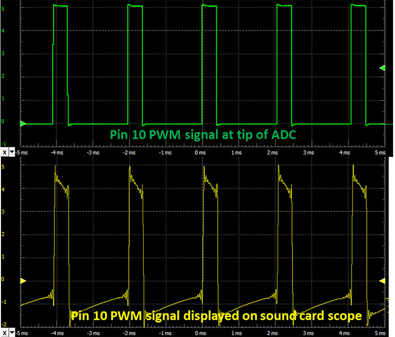
FIGURE 11. Measured PWM signals on pin 10 using the two different instruments. The sound card scope measured the same pulse amplitude, frequency, and duty cycle as the Analog Discovery scope.
I added two measurements to the scopes: the frequency and the positive duty cycle. Both scopes read the same values: 490.3 Hz and 19.6%.
Options for a Higher Performance Oscilloscope
When your project needs good low-frequency response or higher high-frequency response, you have exceeded the limitations of a sound card scope. It’s time to graduate to a real scope. The principles you learn using a sound card scope will directly apply to any other scope you use.
There are many options to choose from, related to:
- Price
- Sampling rate
- Amplifier bandwidth
- Additional hardware functions
- Additional software features
- User interface
- As a stand-alone box or as a USB interface using your PC or Mac
Everyone has their personal preferences, often related to what they have used in the past and for what they feel comfortable. While there are clearly some bad scopes with terrible performance and an equally bad user interface, there are also multiple acceptable scopes in the same price range. If you want to spend less than $50, I recommend finding an old scope on eBay. These are usually better than nothing, but buyer beware.
If you can afford $279, I recommend the Digilent Analog Discovery 2 Scope. This has a sample rate of 100 MS/sec, a 30 MHz bandwidth, a two-channel function generator, and power supply with the same user interface as the sound card scope used in this article. It’s 12 instruments in one.
If you want a stand-alone box scope, check eBay first. If you want to purchase a new box scope, the starting prices are typically about $300 without an integrated function generator or any analysis software. For a scope with significantly higher performance than 30 MHz bandwidth and 100 mS/sec, the prices start at about $500.
All of them have essentially the same user interface you can learn with this free sound card scope. NV
Contact Eric Bogatin
www.HackingPhysics.com
[email protected]
Download the Waveforms Software
https://analogdiscovery.com/download