This article is about an inexpensive magnetometer. The term “magnetometer” is something of a misnomer. The instrument we describe produces a voltage proportional to the magnetic field strength (B) rather than producing an output in magnetic units.
The reason for this is two-fold. First, the instrument can accept one of several Hall-effect sensors, each with its own sensitivity. Second, in many cases, the exact B-value is not of interest. Consider an experiment where the objective is to determine how the magnetic field strength decreases with distance. One would plot B-values against distance and examine the slope.
As another example, one does not need absolute B-values when comparing the relative B-fields of magnets. What is important in these experiments is a linear relationship between the sensor output and the B-field. The magnetometer described in this article is designed for these types of experiments.
Still, a conversion of the voltage to B-values using a reference magnetic field or comparison with a calibrated sensor can be made.
Another feature of the instrument is its basic computer interface, allowing for computer-controlled experiments. Later in this article, I’ll describe how I automated measuring the B-H curve of a metal rod.
Implementation and Circuit Description
As Figure 1 shows, the device is comprised of an Arduino Nano, LCD display, two switches, a DC/DC converter, and three Molex KK connectors.
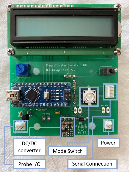
FIGURE 1. The magnetometer device.
Figure 2 shows the Honeywell SS495A Hall-effect sensor probe and assembly that connects to the PCB (printed circuit board).
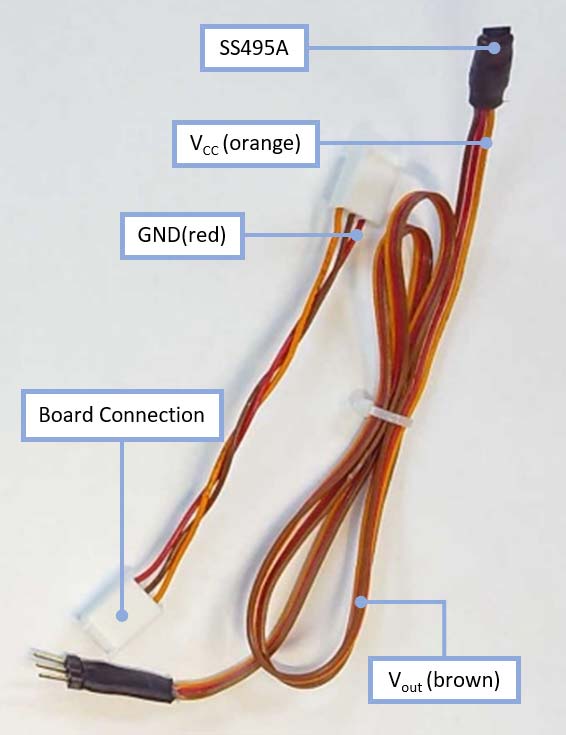
FIGURE 2. Honeywell SS495A Hall-effect sensor probe.
The circuit is powered from a five volt power supply. The overall current consumption is 60 mA and can be powered from a 4xAA battery pack or five volt USB-style power supply. The Schottky diode (D1) provides reverse polarity protection.
To account for different input power supply voltages, the circuit uses the Pololu 791 adjustable step-up DC/DC converter. The output voltage from the DC/DC converter is set to 6.5V which goes to the VIN pin on the Nano. The onboard five volt linear regulator powers the remainder of the circuit.
Pins D2-D5, D11, and D12 (20-23, 29, 30) of the Arduino are connected to a 2x16 back-lit LCD display. The backlight itself is controlled via a toggle switch connected to the power supply, and a 10K potentiometer provides contrast control for the LCD. The mode switch controls how the LCD displays.
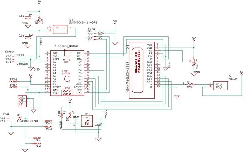
Circuit schematic.
The modes are described later in the article. The pushbutton switch has a built-in LED that is used as a power-on indicator. The serial in/output connector provides access to the Nano serial COM port pins.
Sensor
The Hall-effect was discovered by Edwin Hall in 1879. Figure 3 shows the principle.
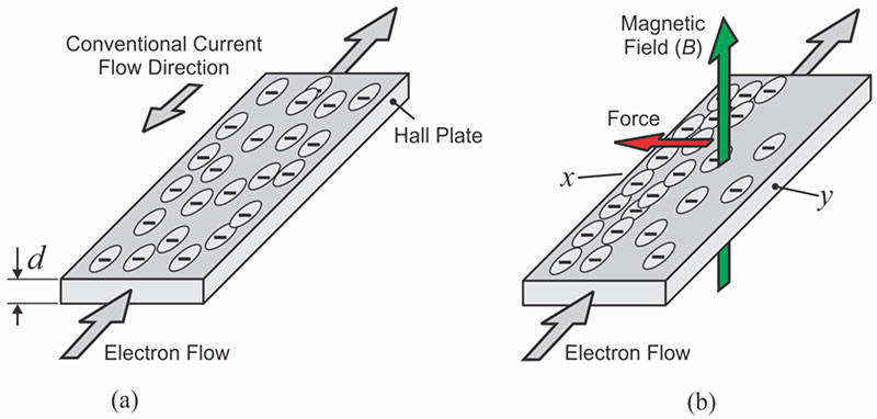
FIGURE 3. The Hall-effect.
When a conductor conducting electricity is placed in a magnetic field, the charge carriers experience a force perpendicular to both the electric field and direction of flow. This causes the carriers to congregate or “bunch up” on one side of the conductor, which results in a small voltage difference. This is the Hall voltage.
While exceedingly small in metal conductors, the Hall voltage is much more pronounced in semiconductors. The Wikipedia page for the Hall-effect provides an excellent demonstration. Today, Hall-effect sensors are widely used as magnetic and current sensors.
Non-contact AC measurements can be made by looping a pick-up coil around a current-carrying conductor. The AC induces a voltage in the pick-up coil which can then be measured. This is the basis of current transformers. A DC (steady) current doesn’t create a changing magnetic field and current transformers don’t work for these currents. However, Hall sensors can generate an output in response to a DC magnetic field. Hall-effect current sensors are widely used where current sensing resistors are inappropriate.
Magnetic Hall-effect sensors are available as ICs that combine the sensing element and signal processing electronics into one unit. These sensors are available with digital and analog outputs. The digital sensor provides a high/low output when the sensed magnetic field passes a threshold. Some applications include magnetic switches and measuring the rotational speed of machines.
Analog Hall-effect sensors are usually radiometric with output voltages that are highly linear with the sensed magnetic field and maximum values directly proportional to the power supply voltage. Therefore, to make precise magnetic measurements requires a regulated power supply.
The sensor in our magnetometer is a Honeywell SS495A radiometric analog sensor (Figure 4).
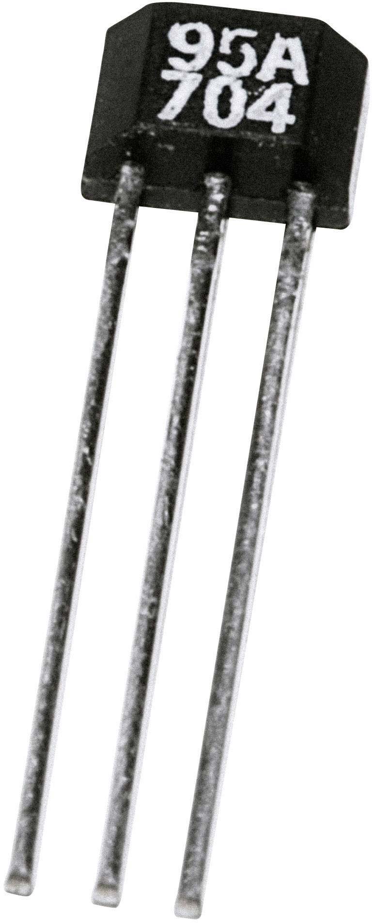
FIGURE 4. The Honeywell SS495A Hall-effect sensor.
Hall-effect sensor sensitivities are normally given in either millivolt per Gauss (mV/G), or millivolt per millitesla (mV/mT). To convert a sensitivity from mV/mT to mV/G, multiply the mV/mT value by 10. The SS495A has a sensitivity of 3.125±0.125 mV⁄G at a 5V power supply. The uncertainty in sensitivity is somewhat large at 4%. The linearity is better at -1.5% and the dependence on temperature is also small at ±0.06%/°C.
The power supply voltage can range between 4.5V and 6.5V, drawing roughly 6 mA. In the circuit, the LM4040 functions as a high-precision zener diode and provides 4.096V. The value of resistor R5 is such that there is enough current to power the Hall-effect sensor and keep the LM4040 zener in regulation. C1 is a decoupling capacitor to keep the power supply “squeaky” clean. The 4.096 voltage goes to the VREF pin on the Nano.
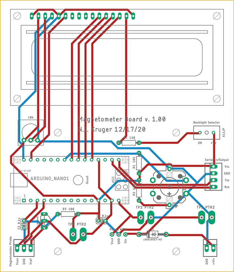
Eagle PCB layout.
As it is radiometric, the SS495A produces an output voltage between 0V and 4.096V. With no applied magnetic field, the output voltage is 2.048V. With a magnetic field in one direction, the voltage increases and saturates at 4.096V in the presence of a strong magnetic field.
When the field is reversed, the output decreases from 2.048 all the way down to 0V in the presence of a strong magnetic field. The output from the SS495A is connected to the A0 (5) pin on the Arduino, which is the Nano’s ADC0 input pin.
Software
The software is reasonably straightforward. We’ll use the LiquidCrystal LCD Arduino library. The pin assignments for the LCD and analog inputs are in the setup block, and the sensor output is digitized, scaled, formatted, and sent to the LCD in the loop block.
void setup() {
pinMode(6, INPUT); // Display mode switch is connected to pin 6
Serial.begin(9600);
Serial1.begin(9600);
lcd.begin(numCols, numRows);
lcd.print(“Magnetometer 1.0”);
// When we start out, display the raw Hall-effect sensor voltage.
ref = 0.0;
state = NO_REF;
// Make the ADC use the reference on the AREF pin. This is a 4.096 V (nominal)
// voltage reference.
analogReference(EXTERNAL);
}
Setup for the device.
The values are also streamed to the Nano serial port. Depending on the state of the mode switch, the output is either 0V to 4.096V or 0V to ±2.048V. By default, the magnetometer updates the LCD once per second.
The magnetometer also accepts three one-character commands through its serial port. The first command is the M (mode) command that preforms the same function as pressing the mode button. The second command is the A (automatic) command that switches the magnetometer to a continuous, one measurement per second mode.
// Communication with RX0
if (Serial1.peek() != -1) {
c = Serial1.read();
switch (c) {
case M: // Mode Switch
if (mode == ‘A’) // Automatic -> Semi-Automatic
mode = ‘S’;
else if (mode == ‘S’) // Semi-Automatic -> Automatic
mode = ‘A’;
break;
case A: // Force Automatic
mode = ‘A’;
break;
case S: // Semi-Automatic
if (mode == ‘S’) // Print Measurement
Serial1.println(str);
else
mode = ‘S’; // Force Semi-Automatic
break;
}
}
else if (Serial1.peek() == -1 and mode == ‘A’) // No Change Needed
Serial1.println(str);
Code for the mode switch.
The third and final command is the S (semi-automatic) command that switches the magnetometer to a manual measure ment mode. When the magnetometer is in the semi-automatic mode, it takes a measurement every time it receives an S command at the serial port.
Sensor Cable
The SS495A sensor is attached to a flat ribbon cable terminated in a three-pin KK connector which connects to the PCB. The ribbon cable is peeled from a standard ribbon cable. After soldering the wires to the sensor pins, adhesive lined heat shrink tubing is slid over the connections and heated.
The result is a sturdy, small, water-tight sensor with a flexible connection to the PCB. The assembly process is shown in Figure 5.
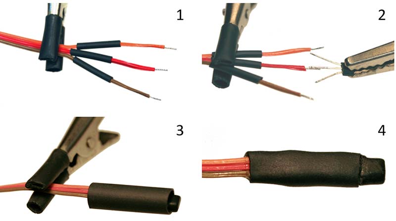
FIGURE 5. The assembly process of the Hall-effect probe.
Calibration
As mentioned in the introduction, the goal of the magnetometer is not to provide measurements in magnetic units (i.e., Gauss) and the outputs are in voltage values. If desired, however, these values can be converted to B-values as follows:
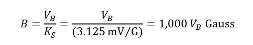
where VB is the magnetometer output and KS is the sensitivity of the SS495A.
If a professional magnetometer is available, one could measure some B-values using both instruments and compare.
Demonstration
To illustrate the utility of the magnetometer, it was used to measure the B-H curve of a short rod of mild steel. Figure 6 shows the setup that consists of the following: a baseplate with two slits for holding the coil in place; a cradle for the steel rod; and a bracket to secure the Hall sensor in place.
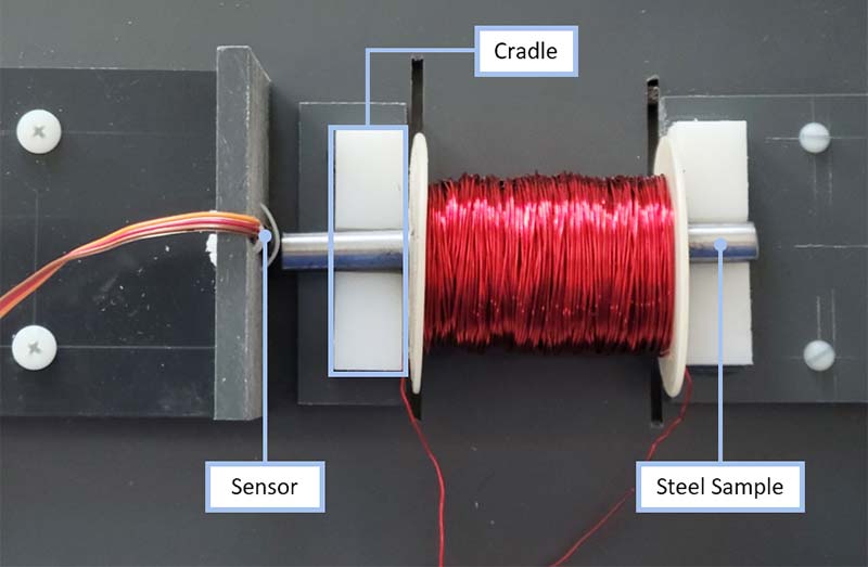
FIGURE 6. A bird’s eye view of the base plate assembly.
The coil consists of 1,313 turns of 22 AWG magnet wire, wound onto an approximately 2×0.8” plastic bobbin.
Figure 7 is a block diagram of the electronic setup.
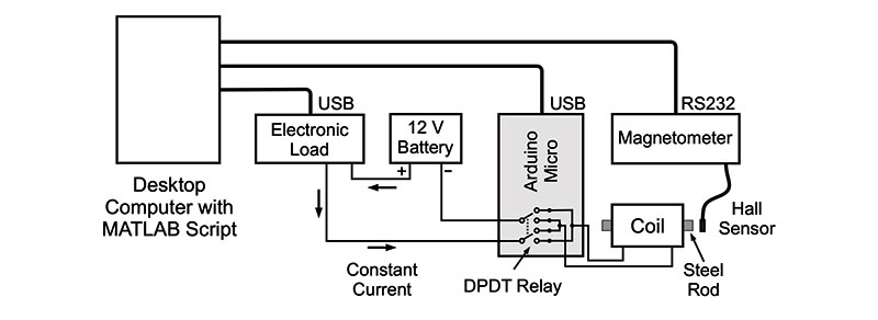
FIGURE 7. A block diagram of the electronic setup. Note the direction of the current.
The magnetometer is connected to the computer via a serial port. A 12V battery and BK Precision 8500 programable DC load are used to force a constant current between 0A and 3.5A through the coil.
This constant current arrangement is needed to combat the effects of temperature rise and the resulting increase in resistance of the coil at high currents. The load is also under computer control.
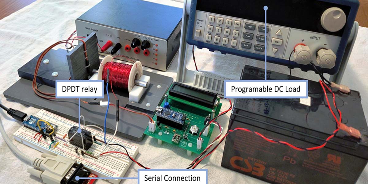
To reverse the current direction through the coil, I used an Arduino Micro to activate a DPDT relay wired for reversing the polarity. This is connected to a third serial port on the computer. A physical overview is shown in Figure 8.
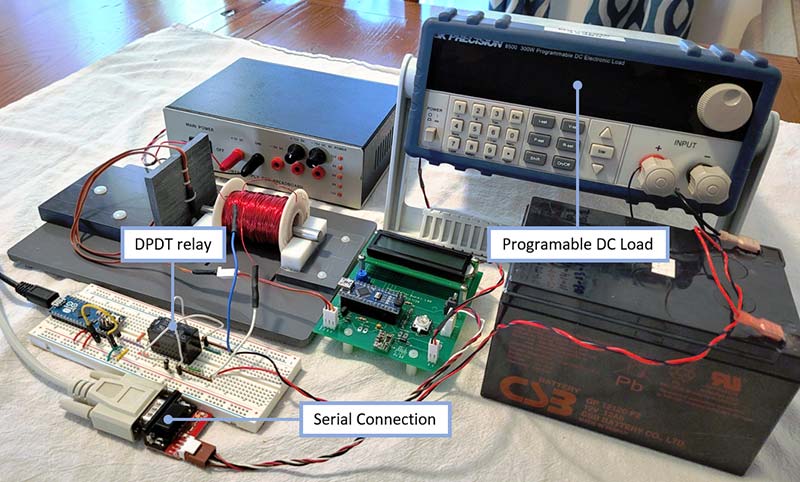
FIGURE 8. The complete experimental setup.
A MATLAB script controls the data collection. It steps the current from 0A to 3.5A in 100 mA steps. Next, it decreases the current in 100 mA steps until the current is zero. Then, the script activates the relay to reverse the polarity, and then it increases and decreases the current as before.
Figure 9 shows the result from an automated measurement made with the setup described.
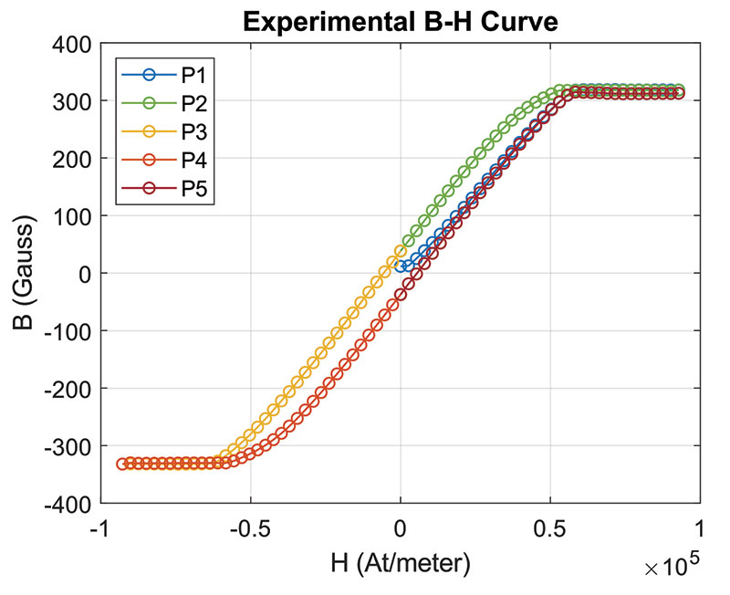
FIGURE 9. Experimental B-H curve. Individual paths are color-coded for clarity.
There are five paths. P1 is the initial magnetization of the rod. B increases linearly with H but around H=0.5x10⁵ At/m, the rod saturates and B does not increase when H increases.
Next, H is reduced (P2), but since the rod’s magnetic domains have been rearranged during P1, B does not follow the same path during P2 as it did in P1.
When H reaches 0, there is a residual B left. Next, the direction of H is reversed (P3) and the magnitude of B increases until the rod saturates at H=0.5x10⁵ At/m. When the magnitude of H is reduced, the curve follows P4. At H=0, there is again residual B in the rod.
Finally, when the polarity of H is reversed and the magnitude is increased, the curve follows P5. A close-up of the BH-curve around the origin is shown in Figure 10.
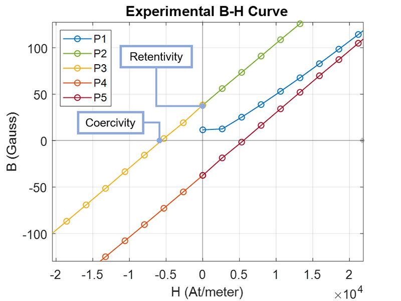
FIGURE 10. A close-up of the B-H curve around the origin to show the coercivity and retentivity.
Conclusion
In this article, we described a Hall-effect based magnetometer. It uses an inexpensive analog Hall-effect sensor, an Arduino, and LCD. The linearity of the magnetometer is surprisingly good when compared against a commercial magnetometer.
The magnetometer can be operated manually or makes measurements under computer control. I then used the magnetometer in a computer-controlled setup to measure the BH-curve of a small sample of magnetic material.
I hope you find this unit measures up to your expectations. NV
Parts List
| Description |
Manufacturer |
Manufacturer Part |
Vendor |
Vendor Part |
| 15-pin Female Header for Nano |
TE Connectivity AMP Connectors |
1-534237-3 |
Digi-Key |
A26425-ND |
| 16-pin Receptable for LCD |
TE Connectivity AMP Connectors |
1-534237-4 |
Digi-Key |
A26426-ND |
| Aluminum Board Standoffs |
Keystone |
8403 |
Digi-Key |
36-8403-ND |
| Arduino Nano |
Arduino |
A000005 |
Arduino |
|
| Backlight Toggle Switch |
NKK Switches |
A11JP |
Digi-Key |
360-2973-ND |
| Brightness Control |
Suntan |
TSR-3386U |
SparkFun |
COM-09806 |
| Capacitor (0.1μ) |
KEMET |
C330C104K2R5TA |
Digi-Key |
399-4387-ND |
| DC-to-DC Converter |
Pololu |
791 |
Pololu |
|
| LCD Display |
Newhaven Display |
NHD-0216XZ-FSW-GBW |
Digi-Key |
NHD-0216XZ-FSW-GBW-ND |
| LCD Standoffs |
RAF Electronic Hardware |
2057-440-AL |
Mouser |
761-2057-440-AL |
| Metal Screws (No. 4) |
|
|
|
|
| Mode Switch |
SparkFun |
COM-10439 |
SparkFun |
|
| Nylon Board Standoffs |
Keystone |
1902F |
Digi-Key |
36-1902F-ND |
| Nylon Screws (No. 4) |
|
|
|
|
| Power Supply Connectors |
Molex |
22232021 |
Digi-Key |
900-0022232021-ND |
| Resistor (100) |
Stackpole |
CF14JT100R |
Digi-Key |
CF14JT100RCT-ND |
| Resistor (10K) |
Stackpole |
CF14JT10K0 |
Digi-Key |
CF14JT1K00CT-ND |
| Resistor (120) |
Stackpole |
CF14JT120R |
Digi-Key |
CF14JT120RCT-ND |
| Resistor (680) |
Stackpole |
CF14JT680R |
Digi-Key |
CF14JT680RCT-ND |
| Reverse Polarity Protection Diode |
Diodes Incorporated |
1N5819-T |
Digi-Key |
1N5819DICT-ND |
| Sensor Head |
Honeywell |
SS495A |
|
480-2005-ND |
| Sensor Input/Output Connectors |
Molex |
22232031 |
Digi-Key |
WM4201-ND |
| Serial Input/Output Connectors |
Molex |
22232041 |
Digi-Key |
WM4202-ND |
| Voltage Reference |
Texas Instruments |
LM4040DIZ-4.1/NOPB |
Digi-Key |
LM4040DIZ-4.1/NOPB-ND |
Downloads
What’s in the zip?
Code Files
Eagle Files