As a final class project for our “Digital Systems Design Using Microcontrollers” course we all took last semester at Cornell University, we created a very unique device. We wanted to design something fun, aesthetically pleasing, and interactive, and since we all enjoy listening to music, we decided on a music visualizer.
Our vision was to create a unit that listens to music being played, then in real time displays a dynamic and colorful visual representation of the music based on the volume and pitch of the notes.
Our music visualizer allows others to experience music through visual means; not only is the display fascinating to look at, but it accurately picks up on the various frequencies that are being played. This is especially useful for people that are hearing impaired, as it allows them to experience music in a new way.
We take sound as input into a microphone circuit which amplifies the audio signal and filters out noise. We then break the audio signal up based on its frequency and amplitude, and map the results to an LED matrix panel.
Design of the Project
First off, let us introduce the brains behind the project: the PIC32 microcontroller. The PIC32 is responsible for running various tasks required for the project: performing the analog-to-digital conversion on the audio signal output from the microphone circuit; breaking this signal into its various frequency components; and mapping these results to the LED matrix display (Figure 1).
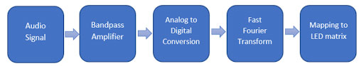
FIGURE 1. High-level design flowchart of our music visualizer.
It appears to run all these tasks at the same time because of threads. Threads are independent processes that the PIC32 microcontroller switches between to run a small chunk of the process at a time. This concurrency allows the PIC32 to run the project.
Music is input into the PIC32 as an audio signal. How exactly do we do this? The first crucial step was to acquire a nice clean audio signal.
We began with a simple microphone circuit and observed the output we were getting from playing music out loud. The output signal was very small, so we next decided to amplify the input.
After testing a range of gain values between 20 and 50, we determined that a gain of 30 was optimal because it was large enough to capture and amplify quieter sounds without causing the input signal to clip for louder sounds. We achieved a gain of 30 by setting R1 to 1 kΩ and R2 to 30 kΩ as shown in Figure 2.
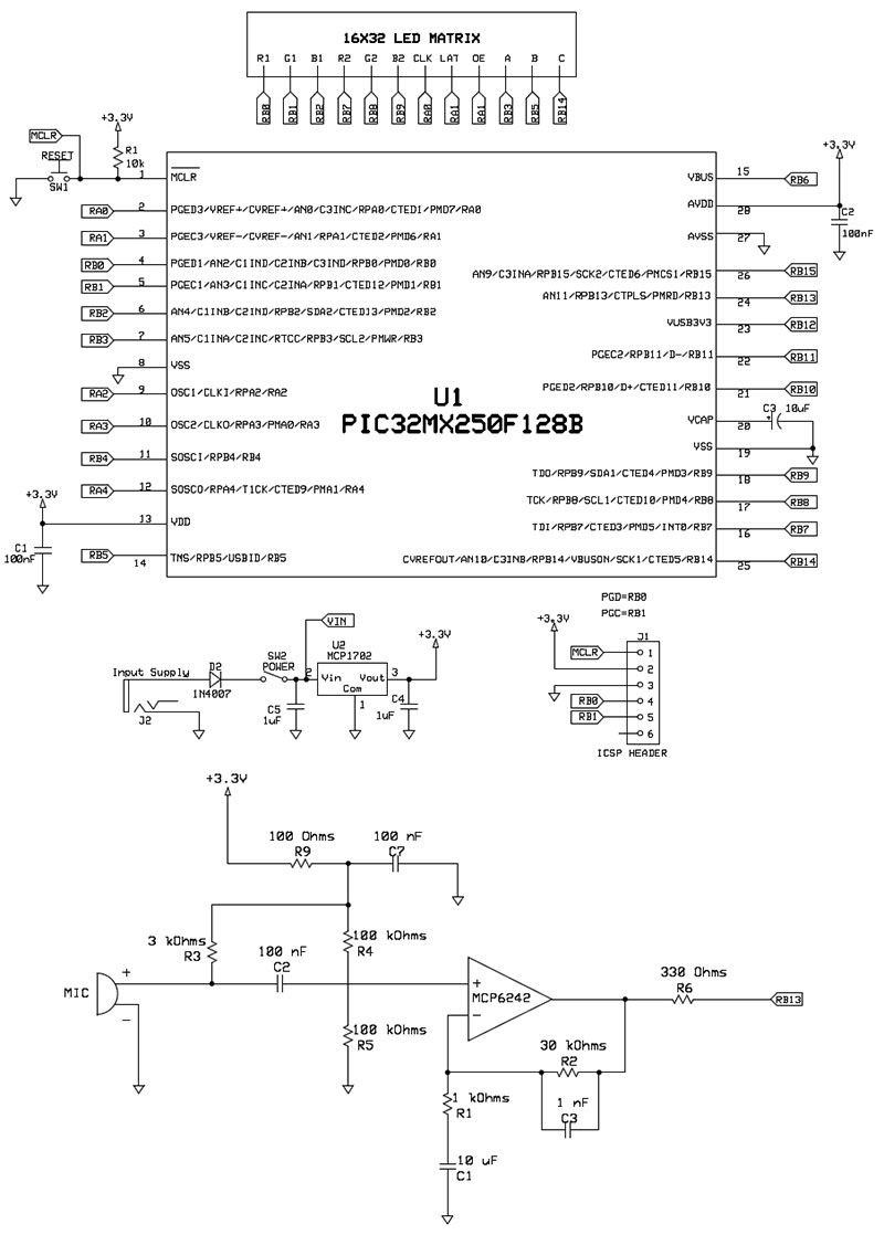
FIGURE 2. Overall schematic which includes connection details for the PIC32MX250F128B microcontroller, the 16x32 LED matrix, and the microphone circuit for amplifying and bandpassing the audio signal. The audio signal was small and noisy, so we created an operational amplifier circuit that removed noise and amplified the signal. We decided to use an electret microphone for audio input, and were able to customize our gain and range of frequencies with a bandpass amplifier circuit.
Once the output signal was significantly larger in amplitude, we noticed it was noisy. The next step was to filter out the noise in the input signal. Since typical voice and instrument frequencies range between 100 Hz and 4,000 Hz, these are the low and high frequency cutoffs we desired for our input signal. We used a bandpass filter to exclude frequencies outside of this range.
One noise source we observed was high frequency interference from the CPU with the analog input. We noted that the high frequency noise came from the power line on the microcontroller. Before connecting the power from the board to the microphone circuit, we low-passed the power in order to reduce the high frequency noise. This power low-pass filter is included in our microphone circuit schematic (Figure 2).
After we acquired a clean audio signal, we needed to sample it using the microcontroller. To do this, we used the analog-to-digital converter (ADC) of the PIC32 which has a resolution of 10 bits. We needed to choose a sampling rate for the conversion.
The majority of energy in music is concentrated below 4 kHz. The Nyquist-Sampling theorem states that in order to avoid aliasing, we must sample at a rate that is double the highest frequency of our signal. So, we sampled at a rate of 2*4 kHz = 8 kHz.
To verify that our sampling rate was not too low, we swept sine waves from 4 kHz to 5 kHz and observed the output on our music visualizer. For loud tones at those frequencies, there was aliasing that could be observed on our music visualizer.
However, when we played a few different songs, we observed that the majority of the energy was concentrated far below 4 kHz, so aliasing was unlikely.
The software behind sampling the output of the microphone circuit is inside an Interrupt Service Routine (ISR). The ISR interrupts the other threads in our program at a rate of 8 kHz to sample the ADC. We store the sampled value into an input array. Each iteration of the ISR, we increment the index into which we put the ADC value. Once the input array is full, we set a flag to notify our FFT thread, discussed below.
Now that we had a discrete signal corresponding to the music, we needed to figure out the frequency components of the music in order to figure out how best to display it. We decided to use the Fast Fourier Transform (FFT) algorithm as it computes the frequencies and amplitudes of the music. Surprisingly, any signal can be represented as the sum of sine waves. The FFT determines which sine waves, explained further in the sidebar.
Fast Fourier Transform (FFT)
The Fourier Series is a way of representing any periodic function as a linear combination of sine and cosine functions. Even the square wave (which looks so dissimilar to a sine wave) can be represented as an infinite sum of sinusoidal waves as shown in Figure A.
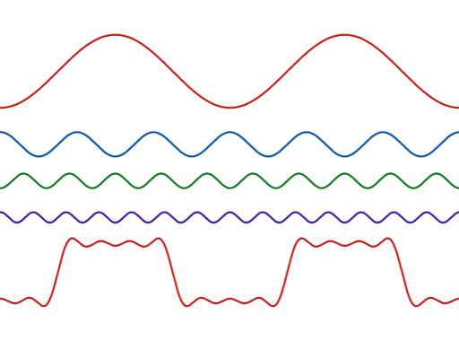
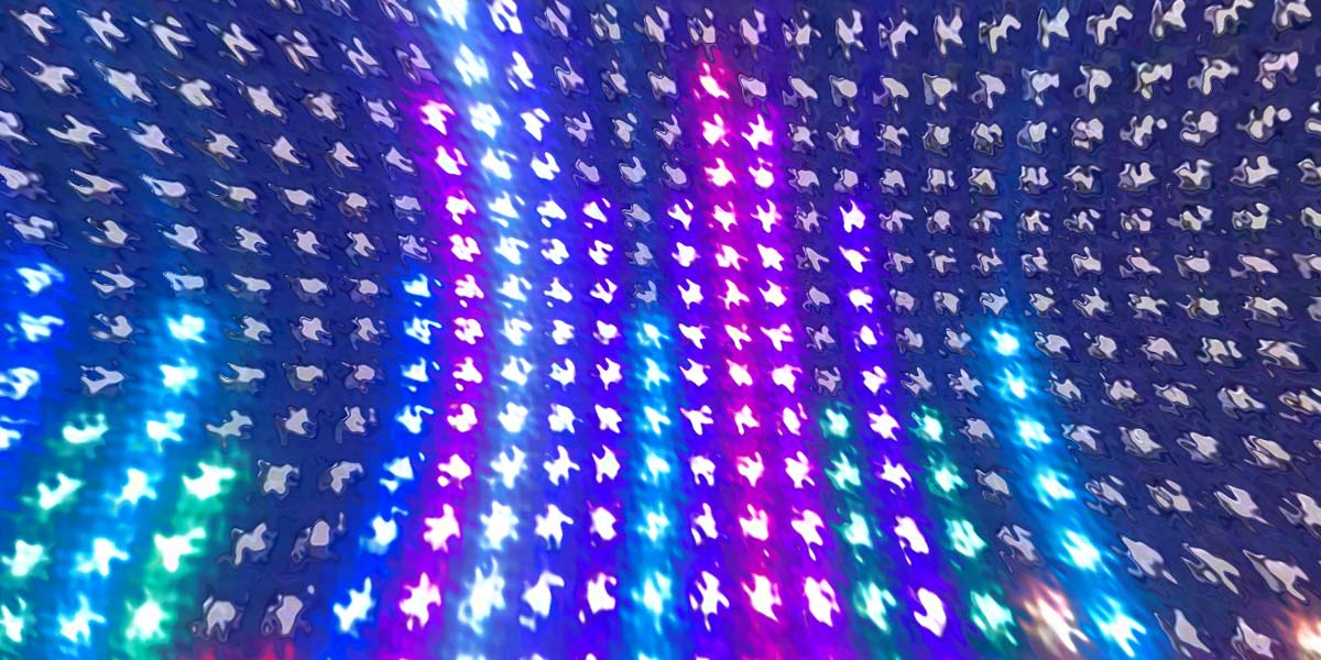
FIGURE A. The LED matrix’s response to a 440 Hz tone.
The Fourier Transform extends the Fourier Series by allowing any function — even non-periodic functions — to be decomposed into a sum of sinusoidal waves of varying frequencies.
Plotting the Fourier Transform of a pure sine or cosine wave results in a peak at the frequency of the wave as seen in Figure B.
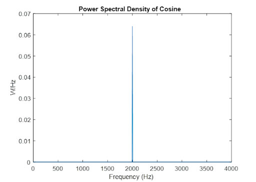
FIGURE B. The LED matrix’s response to a 820 Hz tone.
When multiple sinusoidal waves are summed together, the plot of the Fourier Transform will show multiple peaks; one for each frequency represented in the sum of sinusoidal waves.
For example, the Fourier Transform of a musical chord reveals the frequencies (pitches) of the notes in the chord and the amplitudes of those frequencies (Figure C).
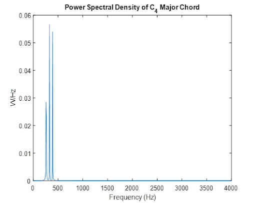
FIGURE C. The LED matrix’s display during “Jingle Bells.”
Fourier Transforms convert signals from the time domain into the frequency domain. The frequency domain representation is a complex-valued function of frequency.
Complex values have a magnitude and phase. The magnitude of the values in the frequency domain represent the amplitude of that frequency present in the signal. The phase in the frequency domain represents the time offset of the sinusoidal wave in the time domain. The FFT is an algorithm that rapidly computes the Discrete Fourier Transform (DFT) by decomposing the DFT matrix into a product of sparse factors. The time complexity of the FFT is O(NlogN) where n is the number of samples.
We dedicated a thread for the FFT computation. We used a lightweight FFT library that computed the FFT in fixed-point rather than floating-point to speed up the calculation at the trade-off of some accuracy. Fixed-point numbers have a fixed number of digits after the decimal point, whereas floating-point numbers have a variable number of digits.
While floating-point numbers can represent decimals with a high amount of precision, they are very slow to do computations on our microcontroller.
In our project, we decided that speed was more important than precision for representing the FFT. Our music visualizer needed to respond quickly to the sound around it.
Our FFT thread waits until the input array is completely filled by the ISR. We compute a 64-point FFT because this transform resulted in 32 bins (groupings of frequencies), which easily mapped to our 32-column LED matrix panel.
Since our sampling frequency is 8 kHz, each bin is centered at a multiple of (8000 Hz/64) = 125 Hz. The top bin is centered at 3,875 Hz.
After computing the FFT, we needed to find the magnitude of each bin. Although imaginary numbers have both a magnitude and a phase, we only calculated the magnitude because that was enough to show the dynamic change in sound, and the human ear is not very sensitive to phase.
The magnitude of each bin is equal to the square root of the sum of the squares of the real (Re) and imaginary (Im) parts of the FFT result in the bin. In our code, we approximate the magnitude using the alpha max plus beta min algorithm, which is:

This approximation has a mean error of 2.4% and a maximum error of 4%. This approximation slightly lowers the accuracy of the magnitudes of the bins, but greatly increases the speed of computation. After the binning is complete, a flag is raised to notify the animate thread which maps the results to the LED matrix that the FFT has been computed and is ready to be displayed.
Once we figured out how to acquire good input and how to transform it into visualizable data, we were ready to display that data. An important design decision was what component we would use for the display. We decided to use a 16x32 LED matrix as it was small enough to be portable, but big enough to express information about the music.
We also made sure to choose an RGB matrix so that we could use color as another way to display more information about the music characteristics. Color in our display corresponds to the volume of a specific frequency range of the music.
We powered this matrix using a 3.3V power supply. The microcontroller could not source the power required for the LED matrix, so we used an external power supply. The LED matrix required — on average — two amps of current. The connections required to drive the LED matrix are:
- R1, G1, B1: The upper RGB pins deliver color data to the top half of the display.
- R2, G2, B2: The lower RGB pins deliver color data to the bottom half of the display.
- A, B, C: The row select lines used to select which two rows of data are currently lit. If using the Adafruit 32x32 LED matrix, there’s an additional D pin to account for the additional rows.
- LAT: The latch signal marks the end of a row of data.
- OE: The output enable signal switches the LEDs off when transitioning to a new row.
- CLK: The clock signal indicates the arrival of each bit of data.
All the above connections were wired to output pins of the microcontroller. In order to drive the LED matrix, we used a library2 that ported the Arduino control code into C.
After we figured out how to power the LED matrix, we moved on to the software side of things. We dedicated a thread to animation: mapping of the FFT output array to the LED matrix.
As explained above, the FFT places the different frequencies into 32 different bins, with each bin containing a 125 Hz range of frequencies. Each bin corresponds with one column on the LED matrix, with bin 0 mapping to the leftmost column and bin 31 mapping to the rightmost column. Bin 0 corresponds to the DC offset; bin 1 is centered at 125 Hz; bin 2 is centered at 250 Hz (2*125 Hz); bin 3 is centered at 375 Hz (3*125 Hz); and so on.
Once we assigned each bin to a column, we picked a height and color to correspond to the magnitude of each frequency bin in the resulting Fourier Transform. The scale we chose for the height of each column was proportional to the log-amplitude. We also mapped color to the height of the column, with each height corresponding to a different color in rainbow color order.
For better visual appeal, we included a gradual decay effect. We saved the previous FFT result and compared its log-amplitude with that of the current FFT result. If, in a specific bin, the log-amplitude of the current signal was less than the log-amplitude of the previous signal, then we changed the log-amplitude to 97% of the previous signal.
If, instead, the log-amplitude of the current signal in that bin was greater than or equal to the previous signal, we kept the log-amplitude as the current signal. This created a dynamic visual display with colored peaks that reacted quickly to a change in frequency, and then slowly fell when a frequency became softer.
The zeroth bin represents the DC signal. In our case, our microphone circuit has a DC offset of 1.5V, meaning that the mean amplitude of the output is 1.5V. Our DC offset is half the voltage of the power source so that we can capture the entire audio signal and avoid any clipping.
Because the zeroth bin represents the DC signal, the magnitude of that bin is always high. The first bin is centered at 125 Hz, but due to the noisy input and an approximate FFT algorithm, the magnitude at this bin was also influenced by the DC offset.
Instead of keeping these bins at a high constant amplitude, we decided to make the second bin 0.9 times the third bin, and the first bin 0.8 times the third bin. This way, the first two bins change in amplitude and the display is more dynamic.
Results
We were very pleased with our completed music visualizer. Not only did the finished device meet our initial design goals, but we were happy with its fast responsiveness to sound and the eye-catching colorful display it produced.
More so, the LED matrix accurately detected and displayed frequencies. We verified frequency detection accuracy first by simply playing single-frequency tones at varying frequencies and checking that the tallest peaks displayed on the LED matrix were occurring in the expected columns.
We first tested playing a 440 Hz tone, utilizing a frequency generator application on a smartphone. The fourth frequency bin is centered at 125*4 = 500 Hz. This bin ranges from 437.5 Hz to 562.5 Hz, so 440 Hz falls into this bin which maps to the fifth column of the LED matrix. When we tested this specific frequency, we did, in fact, see a spike in amplitude at the fifth column on the board as shown in Figure 3.
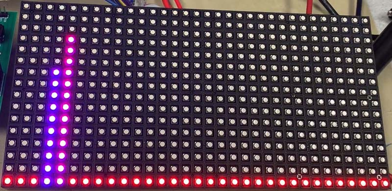
FIGURE 3. A square wave can be approximated by an infinite sum of sinusoidal waves, represented by the following equation: sin(x) + sin(3x)/3 + sin(5x)/5 + ... + sin((2n-1)x)/n. The bottom function is the sum of the top four sine waves. From top to bottom, the functions are sin(x), sin(3x)/3, sin(5x)/5, sin(7x)/7, and the sum of the top four functions.
We also saw a spike in the fourth bin. As 440 Hz is close to the boundary of the fourth and fifth bins and the inherent structure of the FFT can cause spectral spreading, this spike is not surprising.
We reran this test by next playing a tone at 820 Hz. The seventh frequency bin is centered at 125*7 = 875 Hz, and ranges between 812.5 and 937.5 Hz. Thus, 820 Hz falls into the seventh frequency bin which maps to the eighth column of the LED matrix.
When playing the tone, we did confirm a spike in amplitude at the eighth column as shown in Figure 4. We also saw more spectral spreading with the 820 Hz tone.
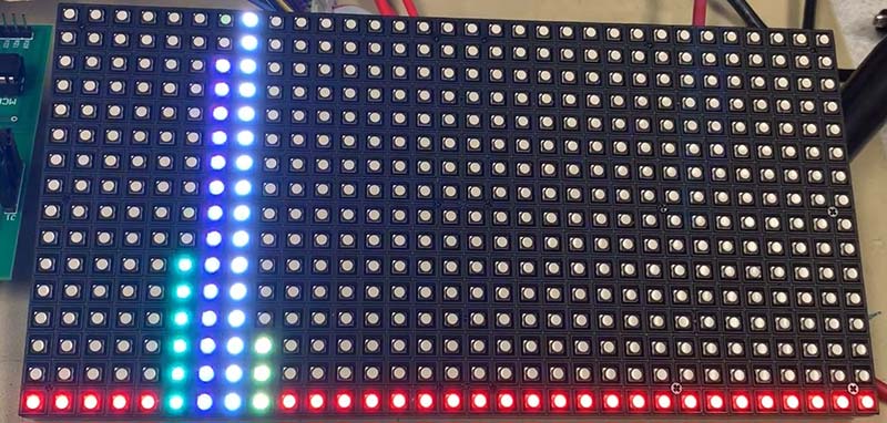
FIGURE 4. Power spectral density of cosine(2000*2πt). Fourier analysis tells us that any signal can be decomposed into a sum of sine waves. The FFT of a cosine wave results in a single peak at the frequency of the cosine wave.
After verifying that our mapping of the FFT algorithm results from frequency bins to LED matrix columns was accurate, we next played a song to see how our display would react to audio featuring different instruments and a wide range of frequencies playing at once. We were blown away by the outcome!
The result was a bright display of fast-changing colors that beautifully complemented the rhythm of the music being played. We also saw how the slight decay we added for any drops in frequencies made the rapid changes in color more pleasing to the eye.
The first song we used to test our music visualizer featured strong guitar and piano melodies and lots of drums and bass, and our display was able to translate these various components into fast-changing movements spanning many columns on the LED matrix.
For the purposes of recording a video demonstration of our music visualizer, we chose to use “Jingle Bells” as our demonstration song because it’s not copyrighted. As seen in Figure 5, the resulting display was just as dynamic and fun to watch. See the video yourself at https://youtu.be/qZ-H_Mc20fU.
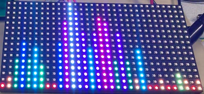
FIGURE 5. Power spectral density of a C4 Major Chord, which is represented by the sum of three cosine signals of the following frequencies: 261.6 Hz (C4); 329.63 Hz (E4); and 392 Hz (G4). As a result, three peaks are seen at each of these frequencies.
Final Notes
Our music visualizer was all-around fun to create and use. Our mapping to the LED matrix and the added decay for visual effect created a dynamic display, which can be customized by anyone. To create your own music visualizer, you can experiment with the display colors. The aesthetics are up to you!
An important design choice was to decide how to convert the audio signal into a visual representation. We decided to represent the music using the Fourier spectrum, as it provided a dynamic display with information about the music’s frequency components and amplitudes.
The X axis of our display corresponds to frequency bins and the Y axis corresponds to the volume of the music in that frequency bin.
An alternate method of music visualization would be to use a spectrogram which displays different time steps of the Fourier spectrum, where the X axis would correspond to time steps and the Y axis would represent the frequency bins. The pixels of the LED matrix would light up a specific color corresponding to the amplitude of the frequency bin at that time step.
We decided to use our visualization axes, as our method carried more information about the amplitude of different frequencies ... a characteristic we found important. NV
Parts List
PIC32/LED Matrix Circuit
U1: PIC32MX250F128B Microcontroller; Digi-Key
U2: MCP1702 Voltage Regulator
R1: 10K ohms
SW1: RESET (Pushbutton Switch); Mouser (474-COM-09190)
SW2: POWER (Slide Switch); Mouser (612-EG1201A)
C1: 100 nF
C2: 100 nF
C3: 10 µF
C4: 1 µF
C5: 1 µF
D2: 1N4007 (Surface-Mount Diode)
J2: Input Supply (2.1 mm Power Jack)
16x32 RGB LED Matrix Panel; Adafruit
J1: M-M Header (shows connections from PIC32 to Microstick II)
MCLR (PIC32) to MCLR (pin 1 on Microstick II)
RBO (PIC32) to PGEDA (pin 4 on Microstick II)
RB1 (PIC32) to PGECA (pin 5 on Microstick II)
GND (PIC32) to GND (pin 27 on Microstick II)
Microstick II (USB Power); Digi-Key
DC Power Supply (5V); Amazon
Microphone Circuit (on separate breadboard)
MIC: Electret Microphone; Adafruit
MCP6242: Op-amp; Digi-Key
R1: 1K ohm
R2: 30K ohms
R3: 3K ohm
R4: 100K ohms
R5: 100K ohms
R6: 330 ohms
R9: 100 ohms
C1: 10 µF
C2: 100 nF
C3: 1 nF
C7: 100 nF
Breadboard; Amazon
Downloads
What’s in the zip?
Code Files
PCB File
Schematics
Complete Parts List
All Necessary Files Related To This Project