Filter Design Software

---

Once you start, it’s hard to stop!

If you’ve ever lived close to an AM broadcast station, you probably experienced the phenomenon known as fundamental overload. It occurs when a receiving device is functioning entirely properly but unable to reject a strong signal. The receiver might be a wireless telephone, a scanner, or even a TV or radio receiver. The AM signal is completely legal but just too strong, disrupting the function of the receiver or overriding the desired programming.

Our Example Filter

Hams often experience fundamental overload on the 160 meter band (1.8–2.0 MHz) which is adjacent to the AM broadcast (BC) band (550 kHz–1.7 MHz). Antennas for those frequencies pick up a lot of AM band RF, overloading the input circuits and creating distortion or false signals inside the receiver. The usual solution is to install a high-pass broadcast-reject filter at the receiver input, attenuating the unwanted AM signals below 1.6 MHz while passing the desired 160 meter signals with little attenuation.

So far, so good, but a filter that doesn’t attenuate signals very much above 1.8 MHz while attenuating them significantly in the adjacent broadcast band is not a simple thing to design. There are tables and equations, but they are tedious to work with. Practically, you’ll need to build the filter with standard-value components as well, and that will affect filter performance too. Sounds like a job for some filter design software, doesn’t it?

There are several filter design software packages ranging from simple calculators to sophisticated CAD programs. Luckily for hams and other experimenters, there are plenty of free or low-cost programs to try (see the sidebar).

---

---

In this article, I’ll illustrate the time-tested and free student version of ELSIE: Design software for passive filters made from inductors (L) and capacitors (C); thus, the name, L-C. By stepping through a sample design, you’ll get a feel for how to turn specifications.

Using ELSIE

Begin by downloading the current version of ELSIE (2.82 as of mid-June 2018) from Tonne Software (www.tonnesoftware.com). Follow the install wizard’s instructions, then run ELSIE. Begin by clicking New Design.

Now it’s time to tell ELSIE what kind of circuit you want. This is the filter’s topology describing the general arrangement of the filter components.

Since we’re designing a broadcast-reject filter for 160 meter reception, we need a high-pass response. ELSIE gives us two choices for high-pass filters: capacitive input and inductive input.

A capacitor in series with the filter at the input (capacitive input) blocks any DC and low frequency signals, so select that topology.

Next, we must select from the many types of LC filter circuits called families — each with a slightly different type of response. For example, the Butterworth family has a very flat response but a gradual roll-off between the passband and the stop band. The Chebyshev family allows some variation in the passband and stopband in trade for a steeper rolloff.

Bessel filters have a constant time delay through the filter in the passband. If you click the ? button next to Butterworth in the Family section, a pop-up window will show the general behavior for each family.

For our filter, we need a very sharp rolloff that passes signals with little attenuation at 1.8 MHz, but with lots of attenuation at 1.6 MHz — the highest frequency of the AM broadcast band at which full-power stations are permitted. (Above 1,600 kHz in the US, AM stations are limited to 10 kW during the day and 1 kW at night. These smaller stations are less likely to cause overload problems than the full-power 50 kW transmitters.)

Chebyshev would be a good choice, but the Cauer family is even better at creating the necessary steep rolloff. The tradeoff is that attenuation of the Cauer filters varies quite a bit in the stopband. That’s okay, as long as we maintain the minimum required attenuation. So, select Cauer as the filter family.

Now, the program needs some performance specifications entered at the right-hand side of the screen. How much attenuation (Stop Band Depth, AS, in dB) is enough for our filter? In my experience, 40 dB is enough to keep even nearby AM stations from clobbering a modern receiver. For Ripple Bandwidth (FC), enter “1.8M” (1.8 MHz) as the lowest frequency of the filter passband. The highest frequency at which we want our 40 dB of attenuation, “1.6M” (1.6 MHz), is the Stopband width (FS).

Filter Order (N) can be thought of as the number of resonances created by pairs of L and C components. The higher the order, the more components are required to create the circuit. Start by entering a filter order of 3 to see if we can meet our design goals.

Viewing the Filter Response

To set up the program’s calculations and display configuration, click the Analysis tab. This is where the inductor and capacitor Q are specified (250 and 1,000, respectively). Lower values of Q result in less stopband attenuation and less sharp rolloff, among other effects. Leave them at their default settings for this exercise. Specify an Analysis start frequency of 0.5 MHz and an Analysis stop frequency of 10 MHz. Leave all other selections and values at their original default settings.

---

---

Before looking at the filter response plot, click the Schematic tab at the top of the screen to show the information in Figure 1. Passband ripple (21.3 dB) and the component maximum/minimum ratios are calculated by the program.

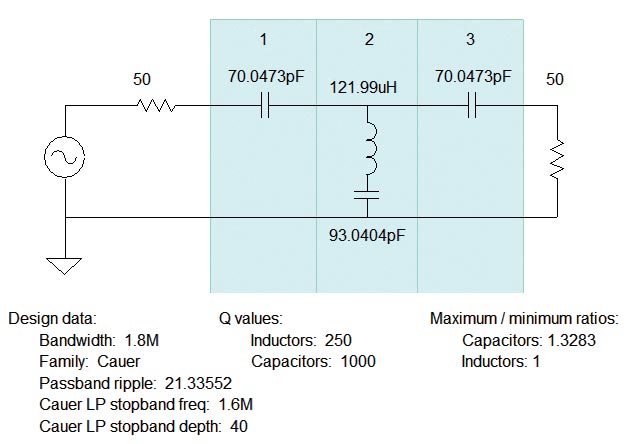
FIGURE 1. The third-order AM broadcast-reject filter schematic and the design parameters used or calculated by the ELSIE program.

---

Now, click the Plot tab for the frequency response graph of Figure 2.

FIGURE 2. Frequency response of the third-order filter shows too much variation in attenuation across the 1.8-2.0 MHz 160 meter band and does not meet the 40 dB attenuation requirement at 1.6 MHz.

---

Place the cursor on the blue response line and hold down the left mouse button. At the bottom of the screen, you’ll see the filter performance at that frequency. The figure shows performance at the response peak of 1.93 MHz.

Move the mouse to the stop band notch near 1.5 MHz to find attenuation there (-69 dB at 1.49 MHz). Attenuation varies by more than 20 dB over the 160 meter band — that’s too much! A third-order filter can’t meet our specifications, so create a higher-order filter. (While you’re at it, use the Design window to select different filter families and compare their responses.)

Interactive Design

This is where the value of easy-to-use design software becomes apparent. Instead of re-starting a laborious design process, simply re-enter new specifications and try again. Return to the Design tab and increase the filter order from 3 to 4, then click Plot. Performance is improved but attenuation still varies by more than 10 dB across 160 meters.

Back at the Design tab, increase the filter order to 5, resetting FS to 1.6 MHz. (The program changes some values when order is changed. Check your settings whenever you change filter order.) This response (Figure 3) is much more useful.

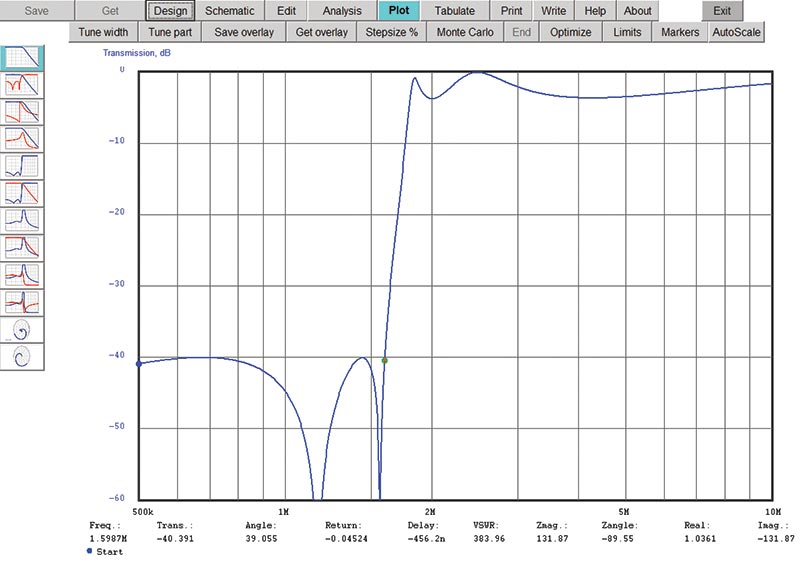
FIGURE 3. Frequency response of the fifth-order filter meets the broadcast band rejection requirement with only 3 dB of variation in the 160 meter band.

---

Attenuation varies by about 3 dB (1/2 S-unit) across the 160 meter band, and we just meet our design goal with -40 dB of attenuation at 1.59 MHz. Click the Save tab to hold on to this design version before proceeding.

Imagine doing this in the “good old days” before the desktop PC became a commodity! For each design, detailed calculations would have to be worked out with a calculator or slide rule at numerous frequencies, then plotted on graph paper if reviewing the full response was necessary. Today’s process takes seconds and allows a lot of “what if” experimentation that was impractical before.

Standard Value Components

The schematic shows all the component values are in a reasonable range. Nevertheless, I don’t think your local component vendor will have, say, 538.436 pF capacitors in stock, nor do you want to have to adjust variable capacitors. Now is the time to redesign the filter using standard fixed-value parts. This will degrade filter performance a bit, but remember that we can continue to work with the design.

Return to the Design window and click the Nearest 5% tab. You’ll be presented with several options, including changing all the components to the nearest standard value in the 5% series.

Other options include just changing the capacitors or inductors, assuming you’ll wind the Ls or tune the Cs. You can also change just the capacitors or inductors, and the program will re-calculate the remaining values exactly so that you can tune up the filter yourself.

Let’s take the easy way out and select the first option to use all standard values. Return to the Design tab, then check the schematic shown in Figure 4.

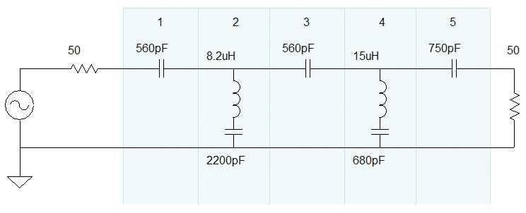
FIGURE 4. The schematic of the fifth-order filter after standard 5% series component values are substituted for exact calculated values. Filter performance is substantially unchanged from the exact value version.

---

How about performance? Viewing the frequency response, not much has changed.

We have a little more variation across the band (now 4 dB), but attenuation at 1.6 MHz is still the same, only failing to reach 40 dB below 840 kHz by less than a dB. This design can be built with off-the-shelf components requiring no tuning to provide useful performance.

Testing a Real Filter

After publishing this design in QST (way back in the January 2016 issue), I received an email from Scott Roleson KC7CJ who built a very nice version of the filter, shown here in Figure 5. He used a sturdy die-cast aluminum box, even making the PCB (printed circuit board) from scratch. The capacitors are silvered-mica with a 5% tolerance. For the inductors, he used miniature encapsulated components.

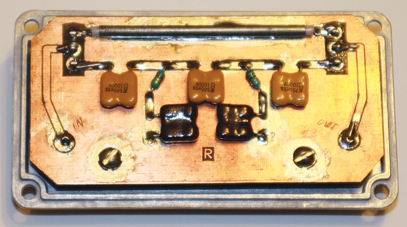
FIGURE 5. KC7CJ’s homemade version of the BCI filter.

---

Roleson created an interesting way of bypassing the filter. Using individual SPDT subminiature toggle switches at the input and output avoided a multi-pole switch that might have allowed unwanted signals to “leak” from the filter’s input to the output through internal capacitance. A piece of aluminum rod has a hole in each end that slips over the switch handles so that both are moved together — simple! Inside the filter, Figure 5 shows the short piece of 50 Ω coax that routes signals around the filter in the BYPASS position.

I set up my vector network analyzer (VNA) to measure his filter’s input-to-output attenuation from 1 kHz (referred to as “zero” frequency) through 10 MHz. Along with Roleson’s version of the filter, I also tested a commercial AM broadcast-reject filter. His version is receive-only and uses components rated for low power. The commercial filter is rated for 300 watts and can be installed in the output of a regular transceiver.

Stopband Attenuation

In Figure 6, you can see there are deep notches in the filter’s stopband. (Compare the as-built filter to the predicted performance in Figure 3 — an important verification step.)

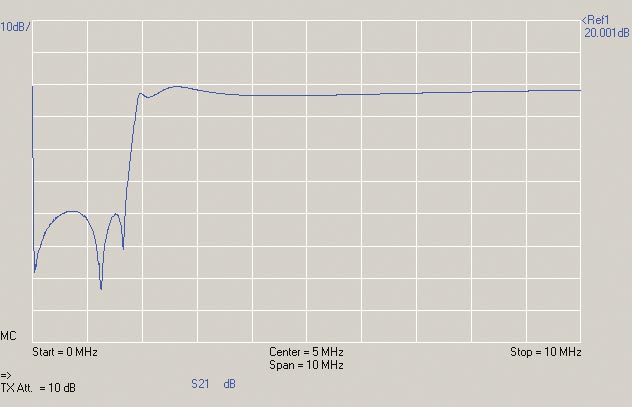
FIGURE 6. The input-to-output amplitude response (S21) of KC7CJ’s filter. The vertical scale (shown in blue at the upper left) is 10 dB/division. The reference level at the top of the graph is 20 dBm. The frequency range is from 1 kHz (given as “0” where a low-frequency artifact is shown) to 10 MHz at 1 MHz/division. “MC” refers to a Master Calibration file having been applied to the measurement. The VNA output (TX level) has been attenuated by 10 dB.

---

That’s okay — we selected a filter family (Cauer) that obtains a steep rolloff by placing notches at strategic frequencies. However, it’s not realistic to give the attenuation of those notches (51, 63, and 58 dB right-to-left) as the filter’s ability to reject AM broadcast (BC) signals.

The stopband attenuation of this filter is measured at the maximum of the two peaks in the stopband, 39 dB of attenuation at about 750 kHz. Did this amount of attenuation satisfy the original design specification for 40 dB at 1.6 MHz? There is plenty of attenuation at 1.6 MHz due to the notch placed there but across the entire BC band, we just barely missed by about 1 dB. Pretty good, nevertheless.

Insertion Loss

A close look at the filter’s response shows that the shape is very close to what ELSIE predicted, right down to the passband ripple between 1.8 and 4 MHz above the filter’s cutoff. Roleson’s filter rolls off a little higher than expected, hitting 10 dB of attenuation at 1.8 MHz. Since this is a receive-only filter, that extra 7 dB of attenuation at 1.8 MHz (we only wanted 3 dB) isn’t a serious deficiency and the filter will work fine.

As the response flattens out, we can see there is about 3 dB of attenuation between 4 and 5 MHz. Similar to how we measure stopband attenuation, this “worst case” attenuation in the filter’s passband is the filter’s insertion loss.

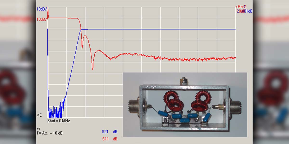
In Figure 7, you see a very different filter response (the blue trace) for the commercial filter. Because it’s expected to be used at 100 watt power levels or higher, insertion loss must be minimized. From the inset photo of the filter components, you can see that larger toroidal inductors are used. These have far lower resistance than the molded components used in the receive-only filter that are wound with very fine wire.

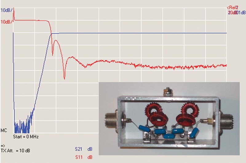
FIGURE 7. The frequency response of a commercial BC-reject transmitting filter. Graph scales are the same as for Figure 6. S21 is the filter’s input-to-output response; S11 (Return Loss) shows the power reflected by the filter at its input and represents input impedance. The filter’s internal construction is shown in the inset.

---

The commercial filter’s insertion loss is less than 0.5 dB from about 2.2 through 10 MHz. The tradeoff is the steepness at which the response rolls off. While the commercial filter has very good attenuation (70 dB) at low frequencies, it doesn’t reach our required attenuation of 40 dB until 1.25 MHz, which is well inside the BC band. This is a consequence of selecting the different filter family, requiring extra components to construct. Sometimes you just have to compromise!

Filter Wrap-up

I hope you enjoyed this short tour through filters and filter design. Filters are one of the most important and widely-used circuits in all of radio at any frequency. Understanding how they are specified and used will make you a better electronics designer, whether you build your own or simply buy them from a vendor.

You’ll find a lot more information about filters for all frequencies in the various amateur radio publications, such as the ARRL Handbook and for VHF/UHF/microwaves in the excellent book from the Radio Society of Great Britain, The International Microwave Handbook. Many hams who have gone on to engineering careers got their start with these two books.

Dive in. The water’s fine! NV

---

---