Suppose you had an electrical oscillator creating a train of pulses, going on-off-on-off-on-off, with a time T between each pulse as shown in Figure 1. It could be from a commercial pulse generator, a 555 circuit, or even an Arduino writing HIGHs and LOWs to a digital output.
The purpose of this article is to ask: How can you determine how well your oscillator is behaving? In other words, what is the oscillator’s (pick one): stability, consistency, performance, accuracy, precision, reliability, etc.?
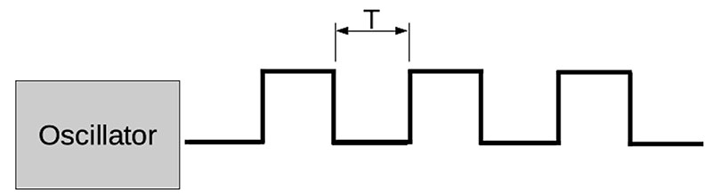
FIGURE 1. A pulse train produced by an electrical oscillator, with a time T between pulses.
In this article, I’ll choose the word “quality,” and will discuss what this means for an oscillator. Then, I’ll demonstrate an interesting instrument that can be used to find Q for a variety of oscillators. For fun, I’ll also show how the same ideas are used to detect muons arriving on earth from the upper atmosphere.
The Idea
Before launching into the crux here, let’s start with a straightforward example of an oscillator that will introduce our technique: a pendulum. Imagine you tie a rock to the end of a string and tie the other end to a high support, like the header in a doorway.
Left alone, the rock will hang vertically from the string. Suppose now you pull the rock back and hold it. Just as you let it go, you start a stopwatch and time how long it takes the rock to swing out, stop, then swing back to your hand (given that your hand remains completely fixed and stable).
Suppose the first time this was done the stopwatch reads 1.0 seconds. If this was a perfect oscillator, you could repeat the swing and get 1.0 seconds again and again and again. Of course, you won’t get 1.0 every time.
You’ll likely get times that resemble those in Figure 2, where some are less than 1.0 and others are greater. Can we assess the stability of the pendulum oscillator from these numbers?
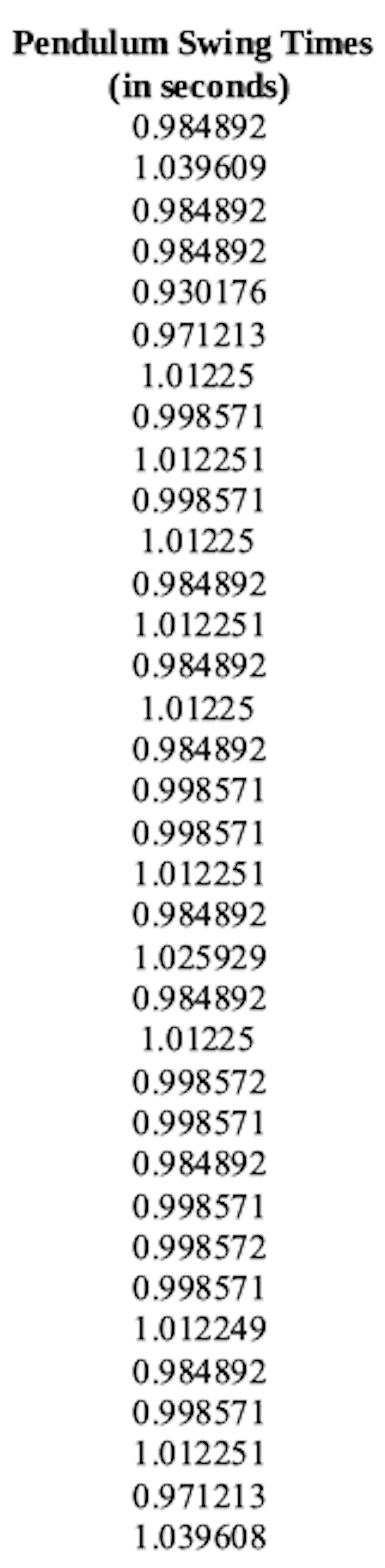
FIGURE 2. A list of pendulum swing times (taken from an actual pendulum).
We can start by applying some basic statistics. Averaging the times, we get 0.998 seconds. So, on average, our pendulum swings out and back in 0.998 seconds, but the average hides the obvious distribution in the individual swing times.
So, next, we can calculate the standard deviation of the numbers, which is 0.02 seconds. (To do these calculations, I pasted the list of numbers into LibreOffice and used the “average” and “stdev” functions.)
What this means is that on average, the pendulum will take 0.998 seconds to swing out and back, and we can expect that 68% of the time a swing will be between 0.996 and 1.018 seconds (± one standard deviation around the average). This is shown graphically in Figure 3, which is a histogram showing the distribution of the swing times.
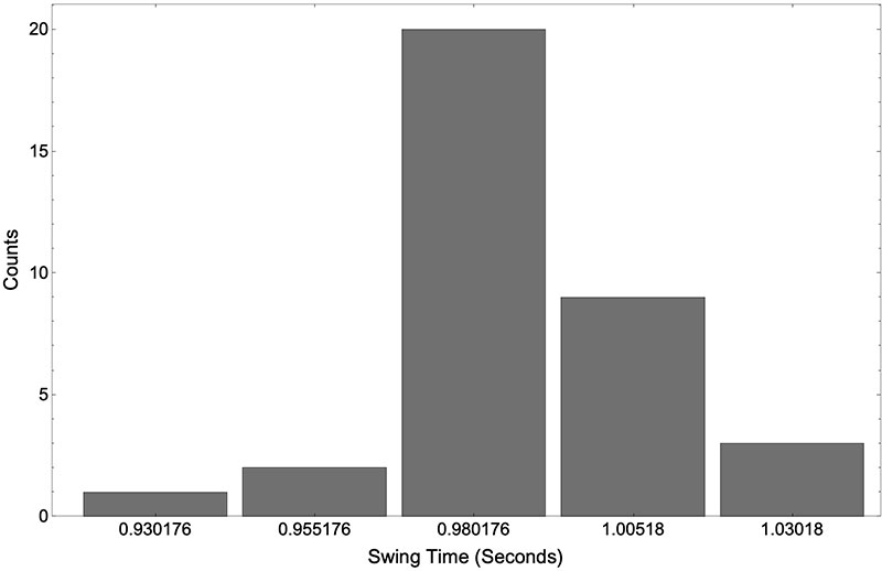
FIGURE 3. A histogram of the times shown in Figure 2. The bin width is 0.025 seconds.
Obviously, a group of swing times around 0.980 seconds happens a lot, but we also get swings near 0.93 seconds occasionally. (This chart was made using the “frequency” function in LibreOffice.)
Now, what about the quality? Well, if we assume that the pendulum’s instabilities are caused by random issues that we can’t control — like air currents, friction, small kinks in the string, etc. — we’ll do one more thing to Figure 3: draw a normal (or “Gaussian” or “bell shaped”) curve over the histogram (using the same average and standard deviation computed above).
As you can see in Figure 4, the Gaussian theory from statistics that describes random “tweaks” to things we measure seems to match up with our histogram. It’s nice because the peak highlights our most expected swing time, while also showing the possibility for other swing times as well (but with lower probability). We acknowledge that our histogram has some gaps in it, but it has an emerging bell shape. We’ll see a more complete histogram shortly.
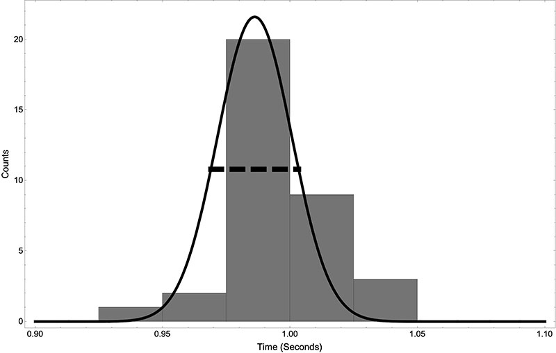
FIGURE 4. A Gaussian fit to the histogram shown in Figure 3.
The Gaussian fit allows us to visualize two important oscillator parameters: the average time; and spread in the times. For the oscillator quality, we’ll need the “full width at half maximum (FWHM),” which is just a little more than twice the standard deviation.
The FWHM is a measure of the spread, deviation, or “sloppiness” of our oscillator. As the name implies, it’s the horizontal width of the Gaussian at the half-amplitude (or maximum) of the Gaussian, and is shown as the dotted horizontal line in Figure 4.
The Quality (or Q) of an Oscillator
The quantity we’ll compute is called Q (yes, “Q” for quality), and is defined as Q=T/ΔT, where T is our average swing time, and ΔT is the FWHM of the swing times. Look carefully at this definition: T/ΔT. So, you take the average swing time (T) and divide it by the spread in the times, or the FWHM.
Our pendulum has an average swing time of 0.998 seconds and a FWHM of 0.047 seconds, so its Q is 0.998/0.047 or about 21. Is this good? Bad? We’ll see.
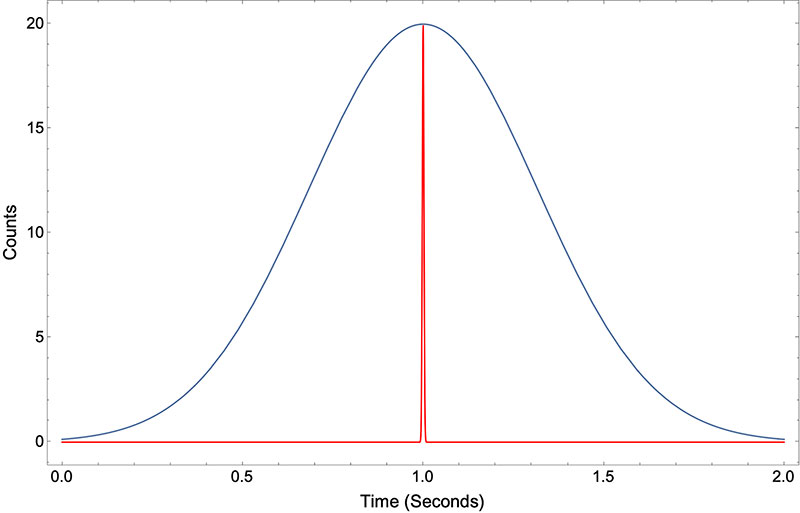
As one more example, Figure 5 shows two hypothetical pendulums, both with an average swing time of around 1.0 seconds. The red pendulum has a very high Q of 190 since its FWHM (or spread) is so small. The blue has a very low Q of 1.3.
 .
.
FIGURE 5. Hypothetical swing time distributions of high (red) and low (blue) Q pendulums.
The red pendulum would show a very regular back and forth motion; it would have a better “quality” than our doorway pendulum.
The blue pendulum would show an awful motion; one could likely just watch it swinging and think “yikes.” It has much lower quality than our doorway pendulum.
The fact that the definition of Q involves both T and ΔT allows us to compare any two oscillators. A 1 MHz oscillator with the same spread as our pendulum, for example, would have a very high Q because its T is so large, but rightfully so. Oscillating at a million times a second with a spread of only 0.047 Hz would be an incredible oscillator! Now on to electrical oscillators.
Electrical Oscillators
For an electrical oscillator, we expect a pulse train coming out as shown in Figure 1. Like the pendulum, our concern will be with T, the time between any two “swings” of the electrical oscillator (or any two pulses produced), and how well the oscillator is able to maintain the T.
In the work here, we’ll find the Q for a pulse train coming from a variety of oscillators: two commercial pulse generators; an Arduino; and a 555 timer. Which do you think will have the best quality? The worst?
The Time to Amplitude Converter
It’s fun to work in a university physics department (as I do) because there’s a lot of cool equipment around. One of my favorites is something called a “time to amplitude converter” or TAC for short. The TAC has two pulse inputs on it, labeled “Start” and “Stop” (see Figure 6).
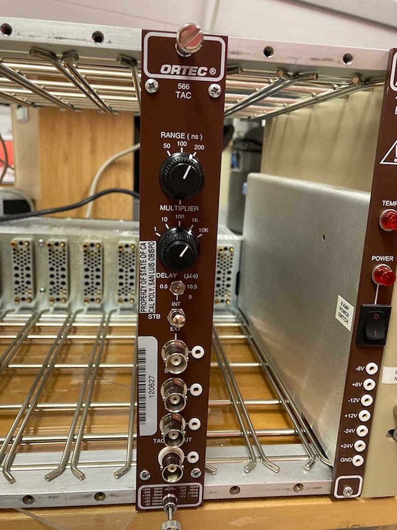
FIGURE 6. The TAC used in this work.
When a pulse arrives at the Start input, an internal timer is started that is stopped when a pulse arrives on the Stop input. When it stops, the TAC will output a voltage pulse, whose height is proportional to the time interval between the start and stop. (Get the name? “Time to [voltage] amplitude converter.”)
This is also a precision device. It has a timing resolution of five picoseconds; is temperature stabilized drifting only by 10 picoseconds/°C change in temperature; and is highly linear in its time to voltage conversion. (Hint: We can trust it.)
I’ve included some oscilloscope traces of the TAC in operation in Figure 7. In each, the upper trace shows two in-going pulses, and the lower shows the output of the TAC. You can see how the output pulse gets larger as the time between the pulses gets larger.
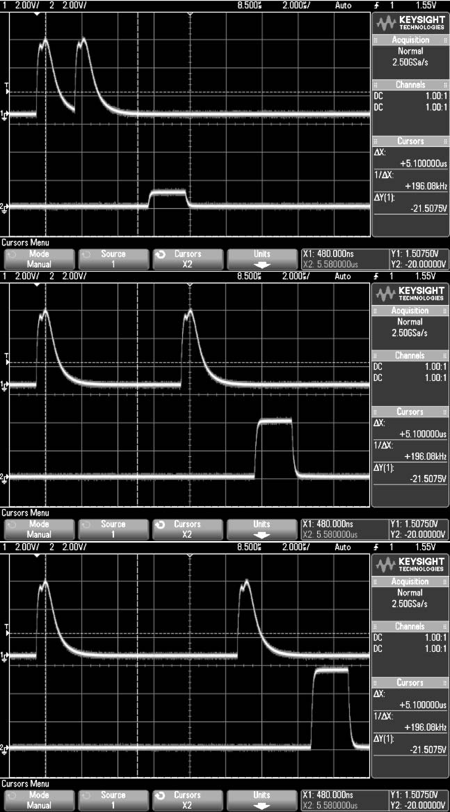
FIGURE 7. Oscilloscope traces of input pulses to the TAC and the TAC’s corresponding output. Upper traces: pulses input to the TAC. Lower traces: the TAC’s output. Notice the output pulse gets larger as the time between the input pulses increases.
In use, the TAC output is sent into a digital-to-analog converter (DAC). Again, being in a physics department, I’m spoiled, as a high speed (100 MHz) 16-bit DAC is available that is able to slice up a TAC pulse into 65,535 (216) different voltage divisions (compare, for example, to the Arduino’s 10-bit DAC).
The software that runs the DAC automatically generates the histograms (like those we made above) in real time (literally, one sees the histogram bars rise upward as an experiment runs). A snapshot of a live histogram of a pulse train going into the TAC is shown in Figure 8.
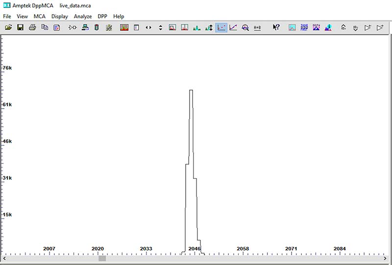
FIGURE 8. A snapshot of a developing histogram taken by monitoring the output of the TAC.
Let the Games Begin
First, I ran a 60 kHz pulse train from a research-grade Berkeley Nucleonics Corp. BH-1 pulse generator into the TAC. This is advertised to have a stability of 0.1% with a temperature shift of 0.03%/°C. (Again, we can trust it.) A histogram of the TAC output pulses for the BH-1 is shown in Figure 9, including a Gaussian fit.
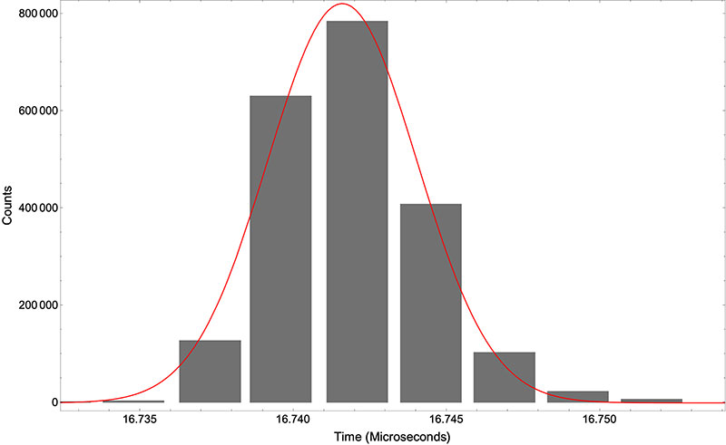
FIGURE 9. A Gaussian fit to the histogram of a research grade pulse generator.
The results? A Q of 2,927! So, over 100x the quality of our doorway pendulum! An old BK Precision 3011 function generator gave Q=2,016. An Arduino (using the code in Figure 10, with pin 3 routed into the TAC) gave Q=2,555. Lastly, a 555 wired in astable mode gave Q=544.
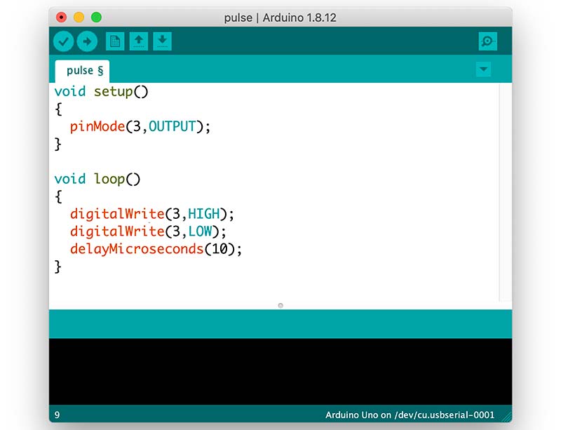
FIGURE 10. Arduino code used to create a pulse train on digital output pin 3.
So, the research grade pulser wins, followed by the Arduino, BK-3011, and coming in last, the venerable 555 (but still beating the 21 of our doorway pendulum).
Notice this oscillator stability business is always done by taking one oscillator and comparing it with another (better) oscillator. Notice the doorway pendulum, for example, was compared with an electronic stopwatch. The electrical oscillators were run against the magical timer inside of the TAC. This shows you how timing assessments are always done: by comparison with some reference that is better than what is being tested.
In the results here, it looks like an Arduino could serve as an adequate tester for 555 circuits and even some bench top function generators. (Future project: make an Arduino Q-meter for pulses coming from a 555 circuit.)
Temperature Stability
The temperature stability of some devices was mentioned above. What is this about? Well, for fun, while the 555 was running, I took my hot-gun (for heat shrink) and heated the air around the 555 circuit to around 130°F, giving the histogram in Figure 11. Look at how the poor 555 shows abrupt jumps in the time between its pulses.
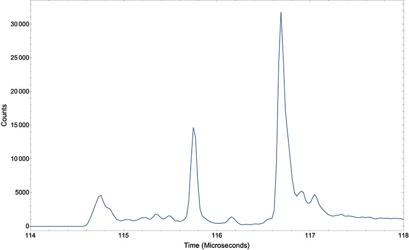
FIGURE 11. A histogram found for a 555 oscillator subjected to (mild) heating by a heat shrink gun.
Nothing against the 555, as every oscillator would show such tendencies. Why? There would be thermal expansion in any capacitor, and resistors are all known to have a temperature dependence. Any transistor in the 555 would experience a gain in its beta and changes in currents flowing between its leads. Therefore, temperature compensation is at least known for our best “absolutes” like the TAC and BH-1.
Muons
Now, what does this have to do with muons? Well, this is what that TAC is used for in the physics lab where I teach. It works like this. When cosmic rays from outer space hit the earth’s atmosphere, muons are created. A muon is like an electron, but 200x more massive. Muons are wispy and hard to detect.
However, if I turn on a detector in the lab, occasionally (about 5x/hour) a muon will stop in the detector and “scintillate” (or generate) a small flash of light.
Now, muons are not stable, and will rapidly decay into a neutrino, antineutrino, and an electron. The neutrinos are lost, but the electron will cause its own flash in the detector. And guess what? The detector is designed to output a pulse when it flashes, just like those shown back in Figure 1.
So, if we feed the detector pulses into the TAC and have the DAC/software pair histogram the time between pulses, what do you think we’ll get? Do muons decay along a very strict and predictable schedule with a narrow high-Q spike? Or, do they decay at any old time, giving a broad low-Q smear in times?
Turns out, neither. We get the distribution shown in Figure 12 (after a two-week continuous run). (Imagine each dot is the top of a bar in a histogram.) The shape is a negative exponential, typical of something that has a “lifetime.”
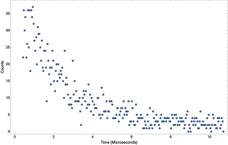
FIGURE 12. Distribution of times between pulses for muon detection.
Such a distribution means that some decays are very rapid (giving a short time between pulses), while other times the decay takes longer (giving longer times between pulses). The average is about 2.2 microseconds — the known lifetime of the muon decay.
Conclusions
So, we’ve seen an unusual way to think about the stability of an electronic pulse train by looking at a histogram of the times between each pulse in the train. Fancy equipment aside, this necessitated the availability of something that had (much) better timing performance than what was being tested.
We also got a taste of the Q-factor, commonly used to assess oscillators. We saw Q values here between 21 and almost 3,000.
A hobby of mine is building wooden pendulum clocks, and my best has a Q of about 300. An inexpensive mechanical watch can have a Q around 1,000. A tuning fork, around 2,000. A crystal stabilized clock can have a Q of up to 100,000 or even 1,000,000. Atomic clocks can have Qs up to 10,000,000 and higher.
All the equipment used here is very expensive, and I’m lucky to have access to it. TACs (also called “time to pulse height converters”), however, do appear on eBay from time to time for under $100. (If you buy one, be sure it can process positive-going pulses.)
You’ll notice back in Figure 6 that it plugs into a Nuclear Instrument Module (NIM) crate for power which you’d also need, but if you can generate ±6, ±12, and ±24 VDC, you could manually jumper the connectors in the back and power it up.
I’d next like to analyze oscillators made from sequenced inverters or AND gates (with the output fed back into the input). The classic two-transistor oscillator would be interesting, as would an oscillator before and after a suitable crystal stabilizer is inserted. NV
Resources
For a nice discussion on Q, see Chapters 4 and 5 of https://tf.nist.gov/general/pdf/1796.pdf.
The TAC used here: https://www.ortec-online.com/products/electronics/time-to-amplitude-converters-tac/566.
The DAC used here: https://www.amptek.com/products/multichannel-analyzers/mca-8000d-digital-multichannel-analyzer.
More on detecting muons: https://www.teachspin.com/muon-physics (note the FPGA timer).
The 555 circuit built is from page 7 of “555 Timer IC Circuits” by Forrest Mims, with R1=R2=500 ohms and C1=0.1 µF.