Above Image Credit: Penn State Lehigh Valley web site.
The most powerful computer in the universe is actually the simplest.
Programmers today are faced with an embarrassment of riches. Software tools are rich and plentiful, and hardware is powerful and cheap. One simple way to measure the ever increasing complexity and sophistication of software tools is to see what it takes to produce a “Hello, world!” program.
In the early days of C and Unix™, it only took a few lines of source code. Now, using a Windows C/C++ compiler or other GUI programming tool, even producing a simple “hello world” program involves hundreds of lines of support code that the application programmer rarely sees.
The programming environments can be large because the machines available today rise in power as they fall in price. Tools are getting easier to use and debuggers are getting more sophisticated. It’s a good time to be a programmer, but sometimes we’re blinded by the power and elegance of our software tools and hardware platforms.
First Principles and Some History
Sometimes it’s worthwhile to step back and look at the world in terms of first principles. Physicists (at least the good ones) view the world from first principles. In mathematics, first principles are called axioms.
It’s refreshing to get away from the everyday routine of cranking out programs and to think about computers in terms of axioms. What do axioms have to do with writing computer programs? Try to answer this simple question: what is a computation?
What is a Computation?
The answer is: The sequence of configurations in a Turing Machine leading to a halt state is called a computation. This means that if your algorithm runs successfully on a Turing Machine, it's a computation. If it doesn't, then it's not a computation!
The world as we know it changed in 1936. The same year the Hoover Dam began generating electricity and Shirley Temple was the top box office draw, a 24-year-old Englishman named Alan Turing completed a paper called “On Computable Numbers” with an application to the Entsheidungsproblem.
Entsheidungsproblem is the German expression for the question of decidability.
What is Decidability?
Decidability means, "Can an algorithm be developed to solve a particular problem that yields a yes or no answer?"
Why the big stink over decidability? Starting in 1910 and lasting through 1913, Alfred North Whitehead and Bertrand Russel published what is considered to be one of the seminal mathematical works, Principia Mathematica. In this three-volume set, Whitehead and Russel attempted to reduce the whole of mathematics to a subset of formal logic. They intended to show that mathematics is complete. The sense of the word complete in this context means that a proof or a formula could be generated by some mechanical means. From an axiom known to be true, other details and conditions can be added to the mechanistic algorithm to create new proofs. This outlook, like in Newtonian physics, offers a clockwork-like, deterministic view of the world. Along came Kurt Godel in 1931 with his Incompleteness Theorem, which effectively showed that the basic notions we hold as mathematical truths cannot be formally proved. This incompleteness applies even to simple numbers. This blew away Whitehead's and Russel's concept of grinding out mechanistic proofs which, in turn, shook the very foundation of mathematics. How could something be decidable if the foundation on which the question is built is incomplete?
In his somewhat obscure paper, Turing described an abstract universal computing machine, now called a Turing Machine.
As it turns out, there is no greater machine, theoretical or real, that equals the capability of a Turing Machine.
The Turing Machine is at the bedrock of modern computer science. Turing’s abstract machine, as he insisted from the start, could actually be built.
Unfortunately, 1936 was also the year that 4,000 Nazi troops quietly slipped into the Rhineland and occupied the de-militarized zone dictated by the Treaty of Versailles, foreshadowing the beginning of World War II.
In 1940, with England at war, and with German U-boats ruthlessly destroying convoy ships, Turing (and other talented mathematicians) were conscripted by the British high command to help crack German military codes.
Luckily, a secret German cipher machine called “Enigma” was captured from a sinking U-boat. With the added bonus of the captured Enigma, Turing cracked the supposedly unbreakable Enigma code and had a significant hand in the Allies winning the war in the North Atlantic.
The unfortunate effect of the war is that it halted the development and materialization of a Universal Turing Machine.
After World War II, a race of sorts between England and the United States to build the first digital computer was off and running. England was building the ACE (Automatic Computing Engine), and the United States was building the ENIAC (Electronic Numerical Integrator And Calculator). Turing was on the periphery of the ACE project and not at the heart of the hardware design, so he turned his thoughts to instruction tables, or what we now call software.
The Standard Turing Machine
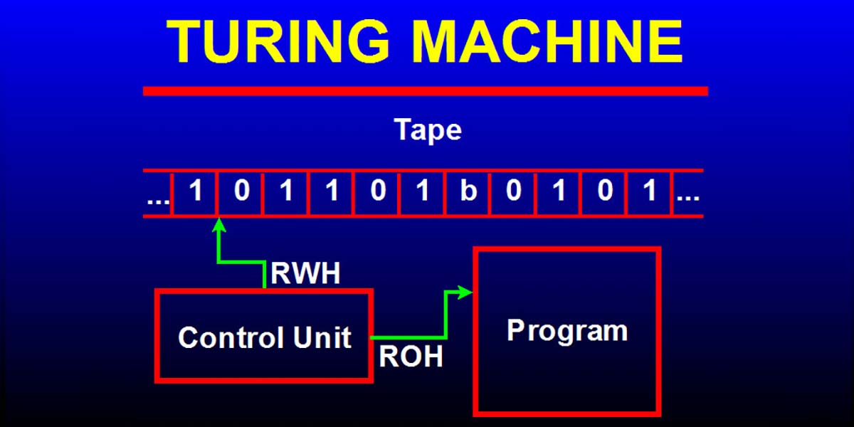
A Standard Turing Machine is shown in Figure 1. It consists of a read/write head and a tape of infinite length that can move right or left one segment at a time. The read/write head reads and writes symbols on the tape.
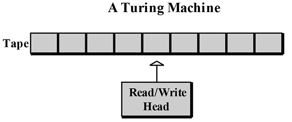
FIGURE 1.
The read/write head, (sometimes called the control head), can read, write, or erase a symbol on the tape segment it is currently under, but only one segment at a time. Believe it or not, this simplest of simple computers is capable of doing anything the most powerful supercomputer can do.
Sooner or later, if you study Turing Machines, you’ll be confronted with formal notation. It’s a little intimidating at first, but it’s really useful and easy to understand. See Figure 2 for an explanation of the Turing Machine symbols.
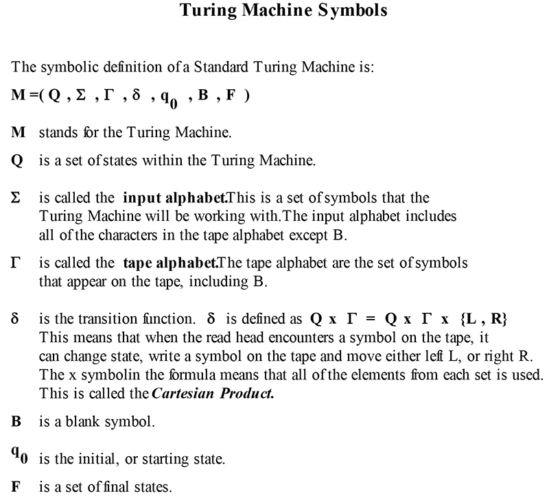
FIGURE 2.
The formal definition of a Turing Machine, denoted as M, is M = (Q, Σ, Γ, δ, q0, B, F).
Here’s what it means: Q is a set of finite states, Σ (sigma) is the input alphabet, Γ (gamma) is the tape alphabet, δ (delta) is the transition function, B is a blank symbol, q0 is the starting state, and F is the final state. Greek letters are used as a notation convention in theoretical computer science, just as they are used in mathematics.
Let’s look at an example so you can get the feel of how a Turing Machine works. Assume we have a tape filled with the symbols a and b and framed by a blank symbol on each end, as shown in Figure 3.
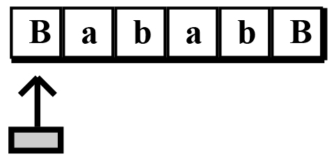
FIGURE 3.
We’ll set the starting position under the left blank. This is the initial state q0. What we want the Turing Machine to do is to change every a to b, and every b to a. We’ll call this Turing Machine the Symbol Exchanger. In order to program the Turing Machine to do the symbol exchange, we need to develop a set of rules, or transition functions, δ. Here are the rules in English, then translated into Turing Machine symbols: Begin at the initial state, q0.
If a blank is over the read head then re-copy a blank on the tape, set the state to the new state q1, and advance the read head to the right. Symbolically, we can write this as (q0 ,B) = {q1, B, R}. In general, this means (State, Symbol) = {NewState, NewSymbol, MoveTo}. Using symbols, we can reduce the long verbal description to a short, precise symbolic declaration. That’s the value in taking the time to learn and manipulate the symbols.
What’s next? The Turing Machine is now in state q1, and now we want the machine to look for an a or b and exchange them, so we need more transition functions. For state q1, if an a is over the read head, stay in state q1, write the symbol b on the tape, and advance the head to the right. This translates to (q1 ,a) = {q1, b, R}. If a b is over the read head, stay in q1, write an a on the tape, and advance the head to the right. This translates to (q1 ,b) = {q1, a, R}.
In order to get the machine to halt in a final state F, we need one more transition function. If a blank symbol B is over the read head, then halt the Turing Machine. This translates to (q1 ,B) = {F}. This transition function is not formally defined when executing a Turing Machine.
In order to get a Turing Machine to halt, there must be a transition that is not defined, so the read head cannot advance to the right or left. All of the transition functions that describe the Turing Machine are listed in Figure 4. Each of our transitions is called a configuration. This is the sequence of configurations that is called out in the sidebar What is a Computation?
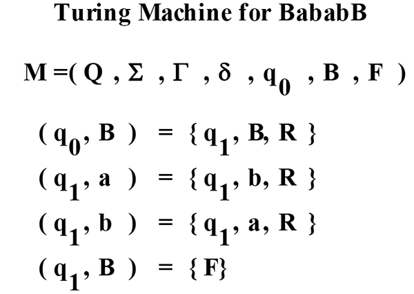
FIGURE 4.
Now we need to run the Turing Machine to see if it works. In most classical Turing Machine literature, a move from one transition to another is indicated by ( . This symbol denotes a running Turing Machine. Figure 5 shows both a graphical and classical representation of our Turing Machine as it runs.
It becomes very cumbersome and takes a lot of space to use a graphical representation for a Turing Machine of any sophistication, so you will hardly ever see them. You will almost always see the classical representation. As you can see in Figure 5, the read head is indicated by the transition functions, q0 and q1. The symbol to the right of the read head is considered to be the symbol under the read head. As the read head reads the tape, it travels right or left and re-writes the symbol on the tape.
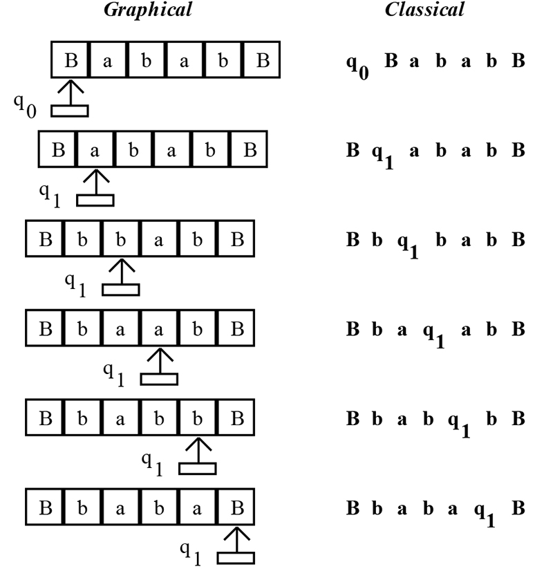
FIGURE 5.
So we’ve shown that our Turing Machine that changes the symbol a to the symbol b actually works. So what’s the big deal? Well, the big deal is that the algorithm to convert one character to another is truly a computation and, since it runs correctly on a Turing Machine, it should run on any conceivable computer in the universe! That’s how deep and profound a Turing Machine really is.
What about adding two numbers together? We know intuitively that it’s indeed a computation, but how do you prove it? See if it runs on a Turing Machine!
One way to express numbers on a tape is to use unary format. In unary format, the number two is expressed as 0110. Three ones are used to represent the number three, and zeros are used to separate the numbers. The number five is unary format is 0111110. We want to see if two plus two is a computation, so the tape will look like B0110110B (don’t forget that the tape is full of blanks, so we have blank symbols reaching into infinity on both ends of the tape).
How can we create a Turing Machine to add these two unary numbers? Look at the tape for a while. The result we want is four, or 011110. If we can shift the rightmost ones to the left one place, we’ll have the desired result. What we need is a form of a shift register.
It’s amazing how much a Turing Machine emulates a modern computer, and it was invented in 1936! Figure 6 shows the transition functions for the adder, and the Turing Machine in action using the classical notation. Run this through the Turing Machine Simulator to verify how it works.
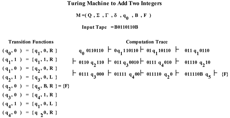
FIGURE 6.
The Turing Machine Simulator TMS
The Turing Machine Simulator consists of three parts: the input tape file, the transition functions file, and the tms.exe simulator. The input tape file is an ASCII text file that contains the tape characters. The transition function file uses a format similar to the classical Turing Machine form. Comments are also accommodated by placing a C at the beginning of a line. With the somewhat cryptic nature of the classical Turing Machine notation, the liberal use of comments is usually necessary (if you want to remember what you did!). A rudimentary parser reads the transitions from the source file and loads the transitions into an array of structures.
What we’ve really built is an interpreter. The transition function file is the program source code, the input tape file is the data, and the tms.exe program is the interpreter. The process of reading a source code file, breaking the source into individual symbols or tokens, then storing the tokens in a data structure is called parsing. Our parser is in the function ReadTuringMachine( ).
To keep the code length short, ReadTuringMachine( ) contains little error checking. This means that the transition function file needs to be reasonably correct, since ReadTuringMachine( ) does not detect syntax errors.
The input tape symbols are load-ed into the InputTape[MAX_TAPE_LEN] array. The transition functions are loaded into an array of TURING_MACHINE structures. The TURING_MACHINE structure and its relationship with the formal transition functions is illustrated in Figure 7.
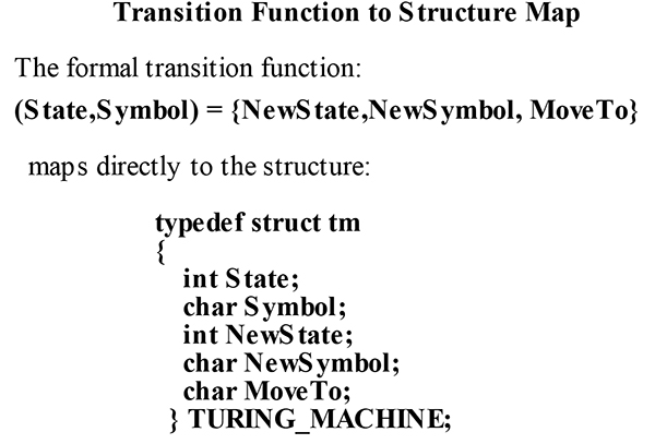
FIGURE 7.
The Turing Machine simulator can be run in Single Step mode, which executes one transition at a time, or in Auto mode, which executes all of the transition functions at full speed. The input tape, transition functions, and computation trace for the symbol exchanger are shown in Figure 8.
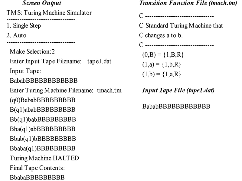
FIGURE 8.
Hopefully, this article has turned you on to Turing Machines. The simple Turing Machine program designed here is just a starting point.
There are multi-tape Turing Machines, Universal Turing Machines, and many other variations. Adapting the TMS program to read multiple tapes would be an interesting project.
Thinking in terms of Turing Machines can be difficult and laborious at times, but the reward is the gained insight into the fundamental nature of computation. It’s fun to write Turing Machines and watch them chug away on the simulator.
Try designing a Turing Machine to copy strings or to do other fundamental arithmetic operations such as subtraction or multiplication. Some machines may be easy to create, and some may be profoundly difficult. Try it and see. Just create an input tape file and a transition function file.
I usually put a .dat extension on the input tape files and a .tm extension on the transition function files. There is no naming constraint, so use your own system if you like.
Want to learn more? There are plenty of web sites that contain detailed, interesting information about Turing Machines, and plenty of transition functions that you can find to run through the simulator.
Remember, out of all of the sciences, computer science is still in its infancy. There are many important discoveries to make and great problems to solve.
Great discoveries are made from the framework of first principles. Using a first principle device, such as a Turing Machine, may aid in the way. NV
Downloads
Turing Machine Simulator Files