Forty years ago in my first job as a researcher at Bell Labs, I bought a data acquisition system capable of measuring two voltage channels to four digits at 100 samples per second. I could store a buffer of 1,000 points in the instrument and suck them out with a computer using the HPIB bus. The very first program I wrote on my HP85 computer was to control this instrument: suck out the data and plot it up.
I measured the voltage increase of batteries as they got colder, and created a voltage vs. temperature plot. Using a linear voltage ramp, I was able to plot the I-V curve of different diodes and match their response to Shockley’s diode equation to better than 1% accuracy.
I paid the huge sum of $15,000 for it. Now, I can build an even more powerful instrument with an Arduino, a shield, and freeware software for less than $100. It measures four input voltage channels at 16-bit resolution, and up to 40,000 samples per second directly into Excel. Once there, I can plot the data in any format I want.
This is a high performance general-purpose instrument that has become the Swiss army knife of my home lab. It is my go-to instrument to measure, record, and display data in just about every experiment I do.
I use it as a data logger, a strip chart recorder, and as an audio signal analyzer. I built a vibration analyzer to measure the impact of damping materials for a fan (see Figure 1).
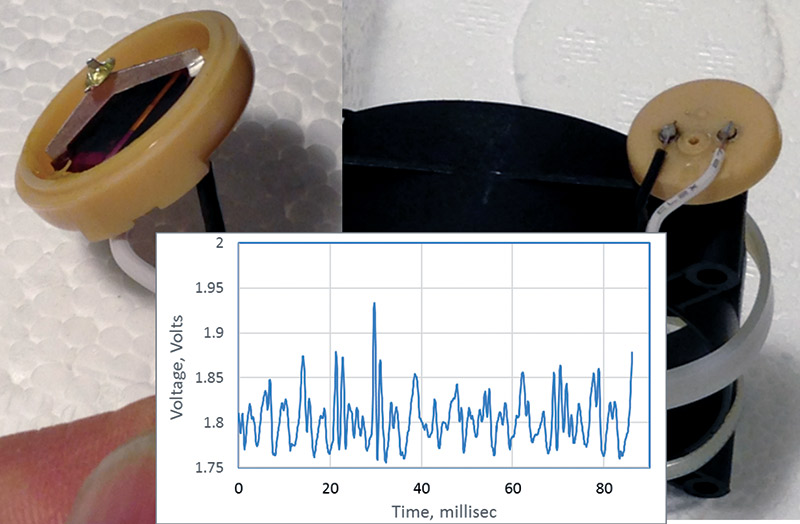
FIGURE 1. Example of a crystal microphone with its foil removed, mounted to a fan. The voltage from the PZT wafer picks up vibrations. The graph has 1,000 measurements during the 90 milliseconds.
With it, I built a micro ohmmeter to measure the typically 20 µΩ contact resistance of a solder joint. I built a noise spectrometer to measure the excess 1/f noise in carbon resistors. I turned it into an impedance analyzer, and fit simple LRC models to the measured impedance profile of any component. I measured the voltage increase of batteries as they got colder, and created a voltage vs. temperature plot. Using a linear voltage ramp, I was able to plot the I-V curve of different diodes and match their response to Shockley’s diode equation to better than 1% accuracy.
These are just some of the measurements this instrument can do. Here’s how you can build this versatile precision data acquisition system.
The Arduino Due Microcontroller
The Arduino family of microcontrollers and boards come in a wide range of price, performance, and form factors. They each have their plusses and minuses. Most of us start out using the Arduino Uno because it is simple, cheap, and readily available. However, when it comes to performance and board size form factor, my favorite Arduino is the Due (Figure 2). I like the Due for three reasons: performance, memory, and form factor.
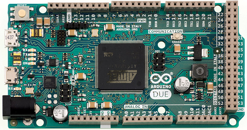
FIGURE 2. The Arduino Due with the standard Arduino pin configuration, plus extra pins.
The Due uses a 32-bit Atmel ARM Cortex M3 SAM3X8E CPU with an 84 MHz clock. This is compared to the eight-bit and 16 MHz clock of the Uno. The combination of higher clock frequency and 32-bit operation means some functions can be more than 20x faster with a Due.
The Due has much more memory, which means larger programs can be written and larger data arrays can be used. A sketch is stored in the Flash memory, while variables are stored in the SRAM memory. The Due has 512K of Flash as compared to the 32K in the Uno, and it has 96K of SRAM compared with 2K in the Uno. I have never written a sketch that runs out of memory on a Due.
When collecting data, the SRAM is important as this is where the variables reside. The largest floating-point array I can declare in an Uno before I get an out of memory error is about 400 elements. In a Due, I can fit an array of more than 500,000 elements before I run out of memory. So far, I’ve never run out of space for data and variables using a Due, but I’ve encountered the limits of an Uno too many times.
While the Due has more digital and analog I/O than an Uno, it retains the form factor of the two rows of pins in the exact same configuration as the Uno. This means the same shields that plug into the Uno can be used on the Due.
In addition to more digital I/Os — all of which can be used as interrupts — there are 12 ADC (analog-to-digital converter) pins, each capable of 12-bit resolution. Its spec says it has 2 DAC pins each at 12-bit resolution, but they are not so useful. Their output swing is limited to a voltage range from 1/6 Vref to 5/6 Vref. When the Vref is 3.3V, this is a range of 0.55V to 2.75V. It’s possible to add a buffer amplifier to turn this range into a 0 to 5V range, but for that effort, it’s easier to just get a good DAC (digital-to-analog converter) shield.
The only slight downside is that the Due runs at 3.3V. We have to be careful what we plug into it. The retail price of a Due is approximately $49 at SparkFun and Adafruit, but less than $20 on eBay (see Resources 1 and 2). The Due has become my first choice for all my Arduino projects.
The Best ADC/DAC Shield I’ve Found
To go with this high performance microcontroller, the Digilent Analog Shield (DAS) is the best analog interface shield I have found (see Resource 3). Its pin footprint matches the standard Arduino footprint and just plugs into the Due (Figure 3).
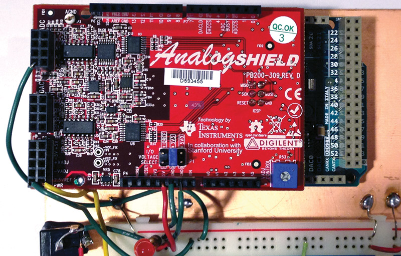
FIGURE 3. Example of a Digilent Analog Shield plugged into an Arduino Due mounted next to a solderless breadboard. This is a powerful combination.
It’s important to move the blue jumper pin located in the bottom middle of the shield to the center position for 3.3V operation. This is one of a number of important tips to follow to get your data acquisition system working the first time (refer to the sidebar).
The DAS uses the SPI bus as the interface to the Due. These are dedicated pins brought out in the center left of the board. A socket in the bottom of the DAS shield plugs directly into the SPI pins of the Due.
This shield has four channels of 16-bit analog input using the TI ADS8343 ADC, and four channels of 16-bit analog output using the TI DAC8564 DAC. The voltage range as input or output for both the ADC and DAC is ±5V. This means each bit level resolution is 10 v/65535 = 0.153 mV.
In addition, there are four DC voltages available to drive analog front-end electronics. There is a fixed ±5V supply, a variable ±7.5V supply, and a fixed high accuracy 2.500V reference. I’ve measured the 2.500V reference with a seven-digit Keithley DMM and found it to be within 1 mV of 2.500V. This is an absolute accuracy of 0.04%. It’s a handy reference to have available — especially for calibration.
Having the other two bipolar power supplies on the shield means we can power analog front-end devices to take full advantage of the bipolar range of the ADC and DAC channels.
I measured the bipolar fixed 5V supply as 4.V and -4.84V when powered by the USB source, and 4.95V and -4.93V when plugged into external power. Since these voltages are regenerated by an onboard regulator, they have a different voltage level and source resistance depending on their power source.
In addition to the voltage level, the other important metric of any power source is its output resistance. This sets the maximum current draw before the voltage drop on the rail is large, like 10% (see Resource 4). Table 1 summarizes the source resistances I measured and their maximum current draw.
| Voltage rail |
Output resistance, W |
Maximum current in mA |
| Adjustable -7.5V |
18 |
43 |
| Adjustable 7.5V |
0.16 |
4,700 |
| -5V |
5 |
100 |
| +5V |
2.7 |
190 |
| |
|
|
| 5V Due |
1.9 |
260 |
| 3.3V Due |
0.55 |
590 |
TABLE 1.
It’s important to note that when using an op-amp powered with the -7.5V supply, the maximum current draw from the devices should be kept below 40 mA. This is not unreasonable. When I use this rail to power other analog front-end components, I always check their current draw and so far, it has not been a limitation (see Resource 5).
The analog shield was created as a joint project between TI and Stanford University. Dr. Gregory Kovacs, a professor at Stanford University, worked with his graduate student, Bill Esposito to design and build this shield as a tool to teach analog design and data acquisition. I hope Bill got an A for this project. He deserves it.
Installation of the DAS with Due
The original library released by Digilent for the DAS and posted on their website is not compatible with the Due. In fact, this library is not very stable even with an Uno. For use with the Due, you should install the library available from Wespro’s GitHub site, last updated on March 24, 2015 at https://github.com/wespo/analogShield (see Resource 6). This library works with the Uno and most other Arduinos.
Initially, I tried the library that Digilent recommended. It never worked very well and gave me hours of frustration. I read through dozens of Arduino forums on related topics looking for a fix, but couldn’t find a solution. Just before I was going to give up and accept that the Due was not compatible with the DAS, I ran across a mention of a library provided by Wespro. I tried it and it worked!
In fact, of all the posted libraries, this was the ONLY library that worked and was stable for the Uno and Due connected with the DAS.
When you go to Wespro’s GitHub landing page, you will see a button in the upper right to “Download the ZIP file.” Click this button and the file “analogShield-master.zip” is downloaded.
Installing this library still in its .zip form is simple. Open the Arduino IDE (integrated development environment) and a new sketch. Under Sketch/include library, you’ll see “add .zip library” (Figure 4).
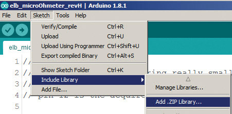
FIGURE 4. Screenshot showing where to find the “add new .zip library” menu item to install the analog shield library.
Click this and point to where you downloaded the analogShield-master.zip file. That’s it. The DAS library is now in your library and you can use it in any sketch. Be sure to close the IDE window and then reopen it. This will ensure the libraries are available.
Every sketch will need at least two libraries with include statements at the top, the SPI library, and the analogShield library. The SPI library is included in the Arduino IDE in every distribution.
It turns out the order in which you list these libraries is important. The SPI MUST come before the analogShield. There are commands in the analogShield library that call SPI commands. At the beginning of each sketch, make sure to use these two include lines, IN THIS ORDER:
#include <<strong>SPI</strong>.h><br />
#include <<strong>analogShield</strong>.h>
This was another issue I struggled with. Some of my sketches worked fine, while others hung up during uploading. The hidden variable was the order of the include statements.
To verify it’s installed and working, open up file/examples and look for the analogShield-master listing. Under it, you’ll see a few example sketches. Click on “ramp.” You can run this to verify your computer talks to your Due and DAS. Just remember to make sure the Due (programming port) is selected under Tools/board, and the correct port is selected and check-marked under Tools/port.
New Commands for the DAS
Two new commands are introduced in this library to read data from the ADC or to write data to the DAC channels. While there are a number of advanced commands, all that is required to get started are the two commands:
- analog.read(chan) — Reads the ADC value of channel “chan” (0 to 3) in units of ADUs
- analog.write(chan, val_adu) — Writes to the DAC channel, “chan,” the value in ADUs
Note that the commands to read an analog voltage from the native 12-bit ADC built into the Arduino Due is analogRead(ID). These commands have a slightly different syntax and so can be used in the same sketch without the possibility of confusion. With the DAS attached, the native analog channels are still available and can be accessed.
The values read or written to the channels are 16-bit integers referred to in units of ADU (analog-to-digital units). For these 16-bit channels, the values range from 0 to 2^16 – 1, which is 65535. In the Due, all integers of any sort are stored as long, 32-bit. When initializing variables, it’s a good habit to always use “long” instead of “int” as this reminds you that they are 32 bits in size.
One nice feature of the DAS is that it is bipolar. The ADC is able to measure voltages from -5V to +5V, and the DAC is able to output voltages from -5V to + 5V. The 65,535 different voltage levels are mapped over this voltage range. Each ADU level corresponds to 10 V/65535 = 0.153 mV.
The native Arduino Due ADC has only 12 bits of resolution — or 4096 levels — spread over a 0 to 3V range. The voltage resolution of each ADC in this case is 3.3V/4095 = 0.8 mV. The analog shield has a resolution that is about 5x more sensitive than the Due, but more importantly, extends over a wider voltage range. This is a huge advantage in giving a larger dynamic range for measurements.
Reading a voltage from channel 0 and placing it into the variable ADC0val_adu is as simple as using the command ADC0val_adu = analog.read(0);. Writing the same value to the DAC channel 0 is as simple as analog.write(0, ADCval_adu);.
Out-of-the-Box Accuracy
As a first test of the accuracy of the DAS, I wrote a simple sketch which averages a bunch of consecutive ADC readings. The scaling is based on subtracting 2^15-1 or 32,767 as the 0 value, and then scaling the ADU value by 10V/65535.
I try to use functions as often as possible in my sketches, and then just call the function in the void loop() whenever needed. As a good habit, I always label functions with a func_ in the front. This makes it obvious what name is a function call or just a simple variable.
This function acts as a simple digital multimeter (DMM) with the four channels. I named this function func_uncalDMM_to_serialMonitor () to indicate this feature. This function is shown here:
<small>void func_uncalDMM_to_<strong>serial</strong>Monitor() {<br />
  // reads voltage on each channel<br />
  long nptsAve_local = 10000;<br />
  long nptsChan_local = 4;<br />
  for (i = 0; i <= nptsChan_local - 1; i++) {<br />
    arrV_meas_nChan_once_v[i] = 0.;<br />
    <strong>Serial</strong>.println(“”);<br />
  }<br />
 <strong> Serial</strong>.println(“attach a voltage to the inputs”);<br />
  for ( i = 1; i <= nptsAve_local; i++) {<br />
    for (i2 = 0; i2 < nptsChan_local; i2++) {<br />
      arrV_meas_nChan_once_v[i2] =<br />
      ((analog.read(i2) * 1.) - 32767 * 1.) * 10./65535.+ arrV_meas_nChan_once_v[i2];<br />
    }<br />
  }<br />
  for (i2 = 0; i2 < nptsChan_local; i2++) {<br />
    arrV_meas_nChan_once_v[i2] = arrV_meas_nChan_once_v[i2] / (nptsAve_local);<br />
    <strong>Serial</strong>.print(“Value for channel “); <strong>Serial</strong>.print(i2); <strong>Serial</strong>.print(“: “); <strong>Serial</strong>.println(arrV_meas_nChan_once_v[i2], 6);<br />
  }<br />
}</small>
I’ve noticed a small bug in the IDE when dealing with integers that are returned in the analog.read(0) command. As long as I only do integer math with the returned value, there are no problems. If I mix integer and floating point, I can get an incorrect calculation unless I first turn the value of the analog.read(0) number into a floating point by multiplying it by “1.” This eliminates any miscalculation error. I use the serial monitor to read the measured voltage on each channel. I connected all four of the ADC inputs together, then to a ground connection, and then to the 2.500V reference on the DAS.
When grounded, the measured voltages in the four channels ranged from -3.7 mV to 7.5 mV. This is a range of about 10 mV above zero.
When connected to the 2.500V reference, the voltages on the four channels ranged from 2.469V to 2.454V. This is a variation between channels of 15 mV with an absolute accuracy about 2%. We may have voltage values reading to 0.15 mV precision, but the accuracy is only to the nearest +/50 mV.
With a simple calibration process, we can do much better.
Calibration
I assume a simple linear connection between the ADU value from the ADC and the voltage it corresponds to. By applying two different well-known voltages (Vref_hi and Vref_lo) and recording the ADU value of each (adu_hi and adu_lo), I can build a simple calibration equation to convert any ADU value into the voltage value. The equation is:
V = V0 + aduValue x Volts_per_adu
I calculate the slope term, Volts_per_adu, from:
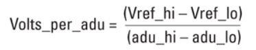
The intercept term, V0, I calculate from:
V0 = Vref_hi – Volts_per_adu x adu_hi
The two reference voltages I use in the calibration are inputs grounded, with 0V and inputs connected to the 2.500V reference.
For each channel, I measure the ADU value at the two voltages and store these in the sketch. Whenever I want to record a calibrated voltage, I use these correction factors and this conversion equation.
After calibration, the absolute accuracy of the voltage recorded is within 1 mV of 2.500V — the limit to the accuracy of the reference voltage. This is now better than 0.1% absolute accuracy.
Getting Data into Excel
Back in June 2015, I wrote an article in Nuts & Volts about using the free tool, PLX-DAQ to suck data from the serial port directly into Excel. This tool was originally written for a Parallax microcontroller, but surprisingly, worked for the Uno. It opened up the use of the Arduino as a real scientific data acquisition instrument. Once into Excel, we can apply the power of this program to display and analyze the real world measurements (see Resource 7).
Unfortunately, I could not get PLX-DAQ to work with the Due. The reset command never got sent to the Due, so it never heard the command to send the data on the serial port. I had come so close to having a really cool data acquisition system using a high performance microcontroller, a souped-up ADC, and the simple yet powerful Excel for data analysis. Unfortunately, I couldn’t get the data into Excel.
Again, I looked over dozens of forums about using the Due and finally, after days of hunting and just about giving up, I found one obscure forum where the solution was posted (see Resource 8). Even now, this link is difficult to find using a Google search, knowing what search terms to use. Its buried in the 758 items returned. Thanks to the heroic efforts of Jonathan Arndt (also known as NetDevil), we now have a freeware tool which works as an open source macro in Excel to read data correctly formatted on the serial port and parse it directly into an Excel spreadsheet. He’s labeled it as PLX-DAQ v2.9.
I can build a simple graph to display the data, and after it is brought in, push the calculate button and there is my data — plotted up (see Figure 5).
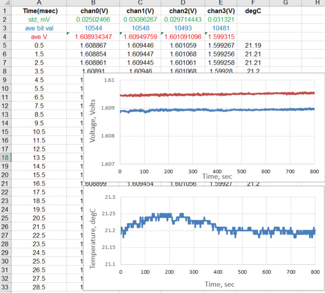
FIGURE 5. Example of the voltage stability of a few AA batteries and the temperature stability in a closed chamber. Note: The voltage scale is 1 mV per division and 0.05 °C per division, over a 13 minute period.
One problem is that the serial port can write data much faster than it can be read into Excel. By trying many different baud rates, I found the highest baud rate I could use to write to the serial port and still read all the data into Excel without losing anything was 15,000 baud. This particular version of PLX-DAQ can read any baud rate, as long as it matches the Serial.begin() value in the void setup() function. The trick to use PLX-DAQ v2.8 effectively to suck the data into Excel even at this slow rate is to turn off the auto calculation. This way, we can still set up graphs and other analysis which will not be executed in real time, but only after all the data is brought in.
If data is written to the serial port slower, it can be brought in and plotted in real time. This is why I created a fast and a slow mode for data acquisition. In slow mode, I get to see the processed data plotted in real time, as it is being taken. I can take measurements on four channels up to 10 Samples/sec and plot them in real time in the spreadsheet. Way cool! Just remember to disconnect the PLX-DAQ v2.9 controller before trying to upload another sketch. It ties up the serial port.
As an example, I grounded all the inputs to the channels, recorded 1,000 data points from each channel as fast as I could, read them back into Excel, and plotted up two channels. In addition, I calculated the average value and standard deviation for each channel (see Figure 6).
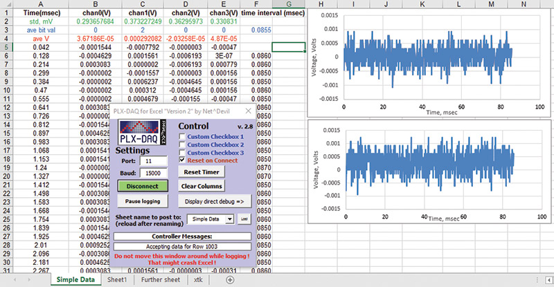
FIGURE 6. Screenshot of the Excel spreadsheet showing the raw exported data and a plot of two channels when the inputs are connected to ground. The plots show the 0.3 mV RMS voltage noise.
This shows the noise floor of the ADC. I measure a DC value of less than 0.3 mV with an RMS value or standard deviation of about 0.33 mV. This is basically ±2 LSB levels.
If I measure the same channel multiple times and average consecutive values, I can reduce this noise. It decreases with the square root of the number of samples. For example, I measured the RMS value of channel 0 with no averages as 0.3 mV. When I measured 25 consecutive samples, I got an RMS value of the noise as 0.057 mV. This is almost exactly 1/5 of the single value noise. It takes 85 µsec to measure four sequential channels. This is an effective data rate of 12 kSamples per second. If I measure just one channel and no averages, I get a sample rate of 43 kSamples per second. This is the limit for this system.
Modes of Operation
What we can do with this instrument is almost unlimited. I find two common modes of operation valuable: fast and slow data acquisition. In fast (or burst mode), data is immediately written into an array as quickly as possible, then is printed out at a slower rate into Excel. In slow mode, the channel voltages are measured and averaged in the Due, and printed into Excel in real time. The fast sketch writes data directly into an array measuring each channel sequentially, and then averaging n different consecutive readings. The algorithm is:
Zero the arrays.
Loop npts2meas.
Measure the time data is taken.
Loop npts2ave.
Loop nptsChan.
Analog.read(each chan).
Add new measurement to previous values of that channel.
Store the sums in the array.
After all the measurements are made, go through each index and divide by npts2ave.
Print the time and value for each channel for each index.
In the slow mode, the same algorithm applies; it’s just that each channel is measured and averaged for a fixed amount of time. The sketches for these different modes are included with the downloads for this article.
An Experiment Example: Temperature Impact on Battery Voltage
One of the first projects I used my data acquisition for was measuring the open circuit voltage of batteries as affected by ambient temperature. I built a simple insulated box with a fan to circulate the air and a TMP36 temperature sensor to measure the ambient air temperature (Figure 7).
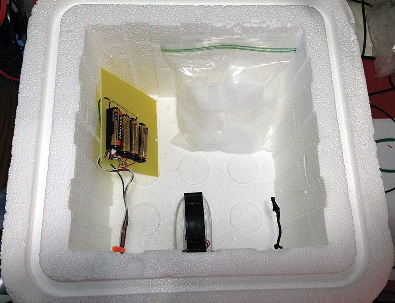
FIGURE 7. Styrofoam box with the temperature sensor and small fan to circulate the air. Four AA batteries were mounted to a small board; a bag of ice was included, and then dry ice was added to cool the air.
Inside this box, I placed four fresh AA batteries and brought their voltages out of the box to measure with the four channels of the ADC. I measured the temperature channel with one of the Arduino Due native ADC channels. The TMP36 sensitivity is 10 mV/°C. With a native resolution of 0.8 mV, the temperature resolution is 0.08°C. This is further reduced with averaging.
I naively expected the battery voltage to decrease with lower temperature. In fact, I saw the opposite. The battery voltage increased with lower temperature. Note, this is with the batteries open circuited and no load (Figure 8).
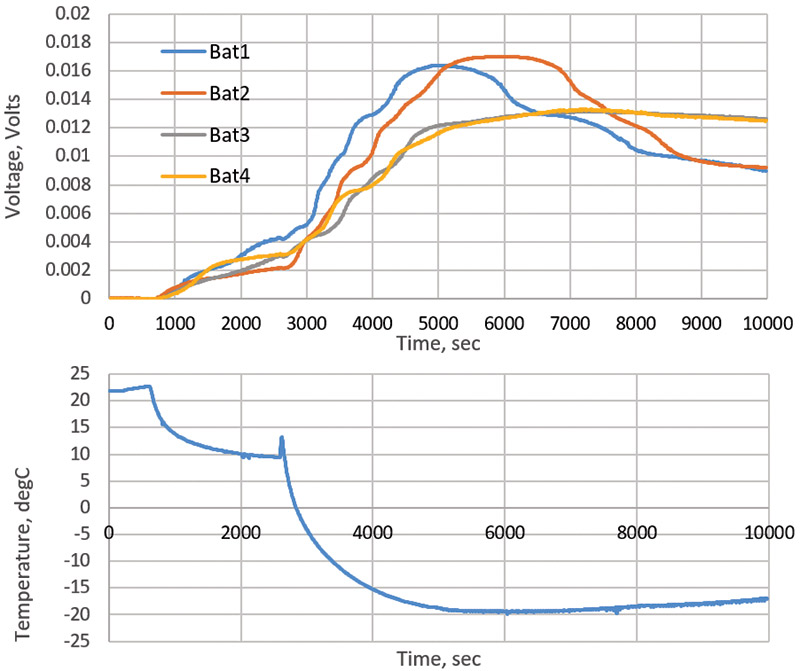
FIGURE 8. The measured changes in the voltages of the four AA batteries and the measured air temperature inside the Styrofoam box.
I put a bag of ice in the insulated box and watched the temperature in the air cool down. As it cooled, I measured the voltage of the four batteries and sampled the data once every five seconds, averaging during this period.
After 45 minutes, the temperature only fell to about 10°C, and it looked like it wasn’t going much lower. During this time, I saw a small increase in the battery voltage of about 4 mV out of 1.6V. This is a 0.25% increase. In this application, the large dynamic range of the Digilent analog shield with averaging is essential.
I really wanted a lower temperature. I just happened to have some dry ice lying around, so I opened the box and threw in a bag of dry ice. The temperature dropped to -20°, stayed there for a while, and as the dry ice all sublimated, the temperature began to creep back up. It’s interesting to note that the temperature of dry ice is -78°C, so if I had had more available, I could have gotten to a much lower temperature.
As a special precaution, whenever using dry ice make sure the room is well ventilated. The dry ice is really CO2. As it evaporates, it will fill the room with CO2. Not safe.
The battery voltages mostly tracked the temperature, increasing by as much as 18 mV in dropping the 40°C from room temperature. It’s interesting to note that of the four batteries, two behaved identically while the other two had a slightly different behavior. All four came out of the same box.
It took me about an hour to instrument this insulated box and about 15 minutes to modify my standard sketch to set up this experiment and start taking data. This is a simple example of how I use this Swiss army knife/laboratory grade data acquisition system as a building block for all of my important measurements.
And now, you can use it too.
One of the nice features of both the Due and the DAS is that they are relatively robust to ESD sensitivity. This has been repeatedly tested by my lab assistant, Maxwell (Figure 9). NV
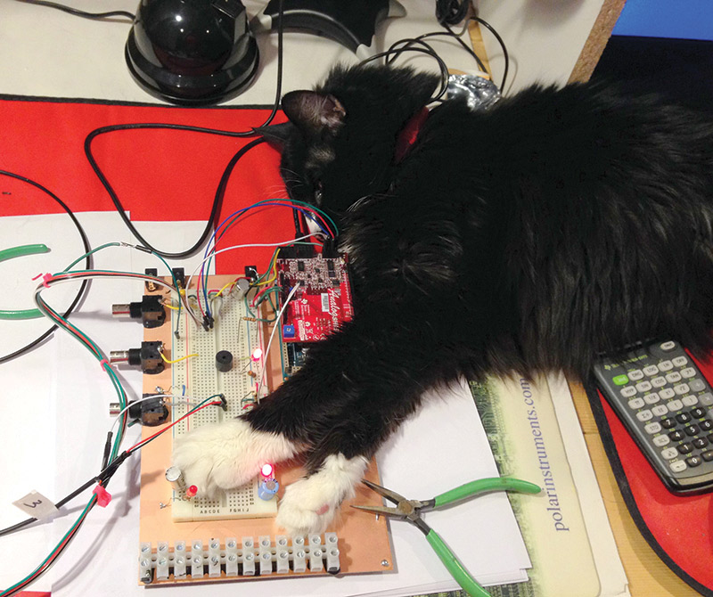
FIGURE 9. An example of one of the many ESD sensitivity experiments Maxwell has conducted, illustrating just how robust this powerful data acquisition system is to environmental stress.
Resources
Purchase Due at Sparkfun
https://www.sparkfun.com/products/11589
Purchase Due on eBay
www.ebay.com/itm/DUE-R3-Board-SAM3X8E-32-bit-ARM-Cortex-M3-Control-Module-USB-Cable-for-Arduino-/331596323040
The Digilent Analog Shield
http://store.digilentinc.com/analog-shield-high-performance-add-on-board-for-the-arduino-uno
See Bogatin, Eric, “Power Sources: The Good, The Bad, and The Ugly,” Nuts & Volts, July 2015.
See Bogatin, Eric, “Why You Need an Analog Front-End and How to Set it Up,” Nuts & Volts, February 2016.
Download the Arduino Shield Library
https://github.com/wespo/analogShield
See Bogatin, Eric, “Arduino Based Data Acquisition,” Nuts & Volts, June 2015.
Link to the PLX-DAQ v 2.9:
https://forum.arduino.cc/index.php?topic=437398.msg3160058#msg3160058
Eight Tips to Get Your System Working the First Time
- Be sure to select the 3.3V pin on the DAS, using the blue jumper in the lower middle pins.
- Download the DAS library from wepro’s GitHub, NOT the Digilent released library. No other library works with the Due.
- After installing the new library, be sure to close the IDE completely, then re-open it so the library is available.
- Be sure to add the #include SPI.h, followed by #include analogShield.h.
- Be sure the Arduino Due (programming port) is selected under Tools/boards and the correct COM port for the Arduino Due (programming port) is checked.
- Download the latest version of PLX-DAQ v2.9 from http://forum.arduino.cc/index.php?topic=437398.msg3160058#msg3160058.
- Remember to disconnect the controller before you try to upload another sketch. The PLX-DAQ will hold the serial port until it is disconnected.
- Set your Serial.begin() rate to no higher than 15,000 baud. Try higher rates until you begin to lose data.
Downloads
What’s in the zip?
Arduino source code