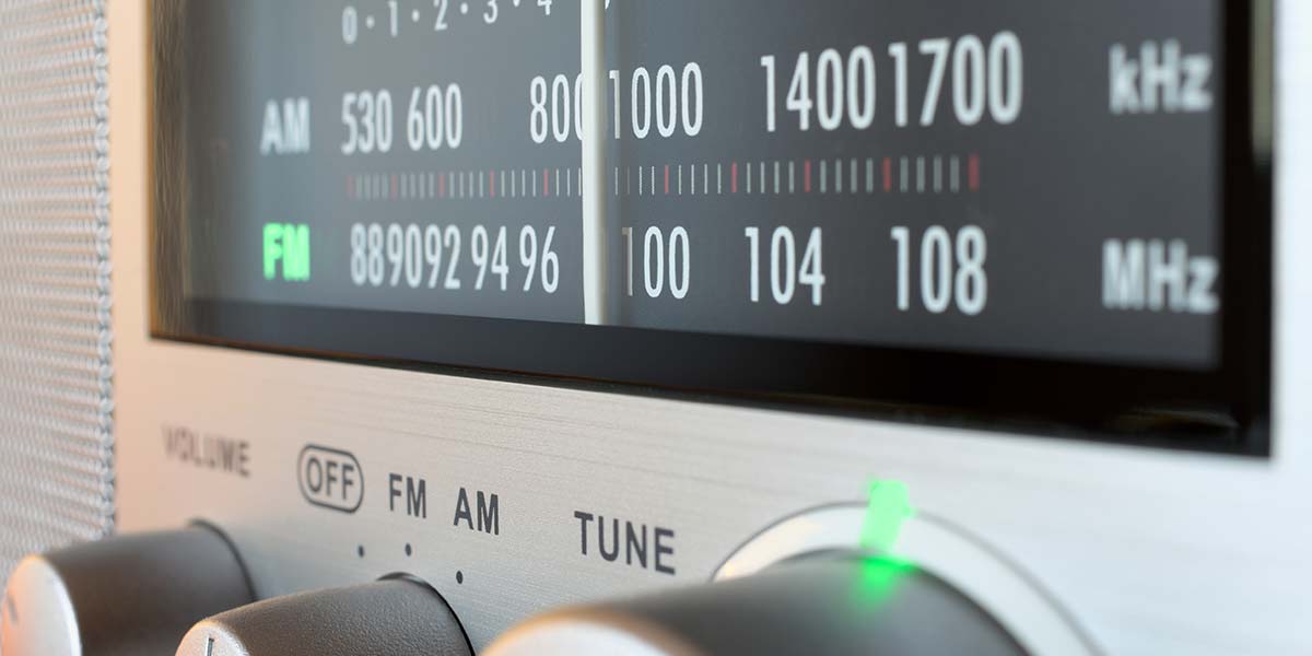
FM Reception with the GNU Radio Companion

» Skip to the Extras

“FM — no static at all” begins the song sung in the ‘70s by the jazz-rock group Steely Dan. This article shows how to combine hardware, software, and your PC to build Software Defined Radios (SDRs) to receive FM radio broadcasts and more.

Stations in the FM band typically broadcast a composite baseband signal that may include monophonic and stereophonic voice and music, subsidiary communications authorization (SCA) services (at one time elevator music, for example), and Radio Data System (RDS) services (providing station and programming information), among some of the possibilities.

Hardware for Software Defined Radios

Appropriate hardware is required to construct software defined radios. Two options — in-expensive and moderately expensive — are discussed here to get you started, but there are many other possible choices.

On the inexpensive side, it’s hard to beat a ~$25 USB dongle that pairs the high-performance R820T digital silicon tuner from Rafael Micro with Realtek’s RTL2832u demodulator/USB 2.0 interface that provides eight bits of resolution. The frequency range listed on the R820T’s datasheet for the tuner is 42-1002 MHz, but most tuners will operate between 24 MHz and 1.8 GHz. The maximum sample rate is about 2.56 MS/s, which will provide a maximum receiver bandwidth of 2.56 MHz. (That’s the reason the designs in this article all use sample rates of 2.4 MS/s.)

The antenna port on most dongles is either MCX or SMA, so you may need an adapter in order to connect to an antenna. Costing approximately ~$100, the RSP1A from SDRPlay is an example of a more capable — as well as more costly — hardware solution. The RSP1A covers from 1 kHz to 2 GHz with up to 14 bits of resolution and sample rates up to 10.66 MS/s. That’s the equivalent to a maximum receiver bandwidth of 10.66 MHz.

The Resources section provides links to several suppliers of this hardware. As far as antennas go, in urban areas, an FM dipole or even a few feet of wire should be adequate to receive local stations. If you live in a more remote area, you may require an elevated external FM antenna or old-style VHF TV antenna for satisfactory reception.

The complexity and sophistication of the electronic hardware required to recover these signals is beyond the capability of most experimenters. Fortunately, modern digital signal processing software, capable personal computers (PCs), and inexpensive software defined radio hardware can be easily combined to receive the information in these broadcasts.

Software for SDR

GNU Radio is a free and open-source software development environment that provides digital signal processing blocks that implement many signal processing functions, including functions necessary for software defined radio (SDR).

The GNU Radio Companion (GRC) is GNU Radio’s graphical tool that implements digital signal processing using visual depictions known as flowgraphs. GRC is easy to use and easy to learn because there are guided tutorials that provide information to get started (see Resources).

GRC can be installed by downloading it from the gnuradio wiki, or by following the Windows workflow provided by SDRPlay in the downloads section of their webpage. (I used GRC 3.17.13.5 downloaded from the SDRPlay site for the flowgraphs in this article.)

Digital signal processing is computationally intensive, so you’ll probably need a dual core processor so GRC runs smoothly. As a point of reference, the Intel CoreTMi5 processor in my Dell Latitude laptop PC handles the flowgraphs I developed for this article without noticeable latency.

In the US, the FM broadcast band is in the VHF part of the radio spectrum with 100 channels allocated between 88 MHz to 108 MHz that are 200 kHz (0.2 MHz) wide. The center frequency for the first channel is 88.1 MHz, while the center frequency of the last channel is 107.9 MHz. There are 99 spaces between the 100 channels; a fact that will be applied when it’s time to discuss receiver tuning. The frequency deviation of the FM carrier is limited to a maximum of ±75 kHz in order to maintain a 25 kHz guard band between adjacent channels. Fun fact: Every FM channel ends with an odd-numbered decimal extension of either 0.1, 0.3, 0.5, 0.7, or 0.9 because the decimal extension of the first channel is 0.1 MHz and the channels are spaced 0.2 MHz apart.

Let’s look at the composite baseband signal that’s transmitted within FM channels. Figure 1 shows the audio and digital signals that are added together to form the composite signal that is transmitted by the FM carrier.

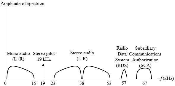
FIGURE 1. FM composite baseband single-sided spectrum.

The first frequency component — 30 Hz–15 kHz — is the monophonic audio channel consisting of the sum of the left and right (L + R) audio channels. The left and right audio channels were summed to maintain compatibility with existing monophonic FM receivers when high-fidelity stereo broadcasts began in 1961.

The purpose of the 19 kHz pilot tone that comes next is to indicate the presence of stereo broadcasts, as well as to provide a coherent reference that can be frequency doubled to 38 kHz to demodulate them.

The next frequency component — ranging from 23-53 kHz and centered at 38 kHz — is double sideband suppressed carrier modulation consisting of the difference of the left and right (L - R) audio channels. This frequency component is demodulated (frequency translated to baseband) by multiplying it by the 38 kHz signal obtained from the stereo pilot tone.

RDS information is broadcast on a 57 kHz subcarrier, which is the third harmonic of the 19 kHz stereo pilot tone. Exactly 48 cycles of the 57 kHz subcarrier are used to encode each bit using differential Manchester encoding to provide a data rate of 57000⁄48=1187.5 bits per second — just adequate enough to encode the song name and station information for the listener.

Finally, SCA subcarriers may be located at 67 kHz and 92 kHz (not shown) and transmit audio information using narrow-band frequency modulation (see sidebar).

Now that we’ve identified the primary signals of interest in the composite baseband, it’s time to implement SDRs that will allow us to receive them.

A few comments about sample rates are necessary before we get started. The sample rate of 2.4 MS/s (set by the variable samp_rate) used by the SDR source blocks must ultimately be reduced (or decimated) to a sample rate that is appropriate for the PC’s sound card (usually 36 or 48 KS/s) connected to the audio sink block. For each block, the sample rate must be kept equal to or higher than the bandwidth of the signal that block is processing for complex samples (blocks with blue ports in Figure 2).

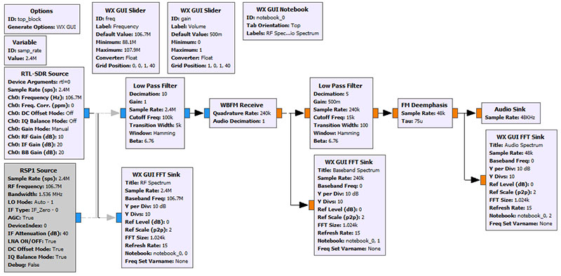
FIGURE 2. GRC flowgraph of an FM monophonic receiver.

The sample rate must be twice as high or higher than the bandwidth of the signal we are processing for real samples (blocks with orange ports). The higher the sample rate, the higher the processing demand on the PC, so it’s important to reduce it as much as possible while still accommodating signal bandwidth requirements.

As a warm-up exercise, let’s build a GRC (GNU Radio Companion) flowgraph to receive monophonic FM broadcasts (Figure 2). This flowgraph shows both RTL-SDR and RSP1 source blocks, but in practice, only the source block corresponding to the selected hardware is necessary. The other source block is either omitted or disabled (shown in gray) in the flowgraph. (Note: After adding the RTL-SDR source block, in the Device Arguments, you may need to add rtl=0 so GRC identifies the connection to the RTL-SDR hardware.)

No hardware? No problem!

I think that one of the most useful features of the GNU Radio Companion (GRC) is the ability to record and play back sample data files. I’m making available two files that I have recorded and uploaded that contain RDS and SCA subcarrier transmissions, along with standard stereo programming.

It’s important to note that the material contained in most radio broadcasts is copyrighted. Fortunately, under the Fair Use Doctrine of US copyright law, it’s permissible to use small amounts of copyright-protected material for non-commercial, educational purposes — which seems to be the case here.

Ready to play back sample data files? All you need to do is follow these four steps:

Download the file(s) from my webpage (see Resources) to your PC desktop.
Disable (or remove) the SDR-RTL or RSP1A Source block and replace it with a File Source block.
Open the File Source block and browse to locate and select the file from Step #1.
Execute the flowgraph. GRC will play sample data from the file instead of from the hardware.

Notice that the File Source block has a “repeat” selection so that the file repeats automatically when it reaches the end of the file.

After adding the RSP1 source block, in the LNA On/Off box, change “0” to “True” or “False” to enable or disable the LNA and correct the error that appears when this block is added. (This does not apply to the RSP1A. I have the RSP1, but the RSP1A is what is available now.) Two GUI slider blocks are used to set the variable values for freq and gain that control the received frequency and audio volume.

Figure 3 shows the slider used to set the value of the variable freq according to the low and high frequencies and channel spacing for the FM broadcast band discussed earlier.

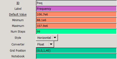
FIGURE 3. Properties for slider setting frequency.

Figure 4 shows the slider used to set the value of the variable gain that controls the audio volume. Also, don’t forget to set the speaker volume on your PC to an appropriate level when the receiver is in operation.

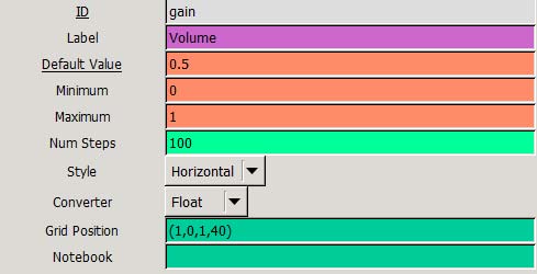
FIGURE 4. Properties for slider setting volume.

Returning to the GRC flowgraph in Figure 2, the FFT plot titled RF Spectrum shows the spectrum received by the selected SDR hardware. Since the sample rate is 2.4 MS/s and the samples are complex, this FFT displays a 2.4 MHz bandwidth of spectrum centered around the value of the frequency variable freq. The RTL-SDR source block also feeds a Low Pass Filter block which serves to select the desired channel and decimates the sample rate to 480 KS/s.

The WBFM block recovers the composite baseband signal and sends it to the second Low Pass Filter block to recover the monophonic audio. The gain of this block is controlled by the variable gain and the block further decimates the sample rate to 48 KS/s.

A second FFT plot titled Baseband Spectrum displays the composite baseband spectrum recovered by the WBFM block. Since the sample rate is 480 KS/s and the samples are real, this FFT plot displays the 240 kHz bandwidth of the baseband spectrum. Finally, high frequencies are deemphasized according to standard FM protocol by the FM Deemphasis block and sent to the Audio Sink block, which makes them audible by sending them to the PC’s sound card.

A third FFT plot titled Audio Spectrum displays the spectrum of the monophonic audio signal. Since the sample rate is 48 KS/s and the samples are real, this FFT plot displays a 24 kHz bandwidth of the monophonic audio spectrum. The Notebook block causes each of the three FFT plots to display using tabs for convenient review during receiver operation.

I think the ability to display actual signals at each step of the receiving process makes GRC invaluable in understanding SDR and radio theory. Figure 5 depicts a sample composite baseband spectrum captured during receiver operation and identifies many of the signals we have discussed so far in this article.

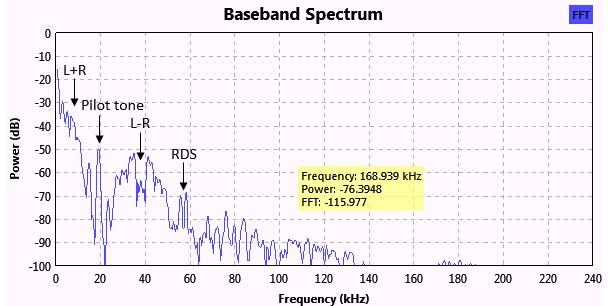
FIGURE 5. Composite baseband spectrum captured from FM monophonic receiver showing: (a) L + R monophonic audio; (b) 19 kHz stereo pilot tone; (c) L - R audio (using double sideband suppressed carrier modulation); and (d) RDS data channel (using binary phase shift keying). (Note: SCA signal is not present in this example.)

Figure 6 depicts the GRC flowgraph for a FM monophonic receiver that includes RDS decoding and display. A complete discussion of this flowgraph exceeds the space I have here, so a few comments must suffice.

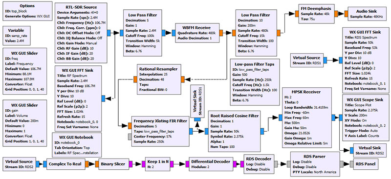
FIGURE 6. GRC flowgraph of an FM monophonic receiver that includes RDS decoding and display.

The monophonic FM receiver shown in the upper part of the flowgraph is identical to that shown back in Figure 2 and functions in the same way. The purpose of the Rational Resampler block is to decimate the sample rate by a factor of 48 and interpolate the sample rate by a factor of 25, which results in a new sample rate of 480k⁄48∙25=250k.

The Frequency Xlating FIR Filter block shifts the RDS signal located at 57 kHz to baseband; filters according to the parameters listed in the Low-Pass Filter Taps block; and decimates by a factor of five to reduce the sample rate to 50 KS/s.

Next, the signal is filtered by the Root Raised Cosine Filter block before passing on to the MPSK Receiver block. In this case, M = 2, so the receiver decodes the signals as binary phase shift keying (BPSK).

The Scope Sink block displays the constellation of the BPSK signal. The Binary Slicer block converts the real-valued sample to a binary value of 0 or 1 prior to being decimated by a factor of two by the Keep 1 in N block. The next three blocks — Differential Decoder, RDS Decoder, and RDS Parser — decode the binary information and format it for display by the RDS Panel block.

Figure 7 shows the BPSK signal constellation and the corresponding station information on the RDS Panel that is displayed during reception. The location and phase reversal of the BPSK signals are clearly apparent in the scope plot.

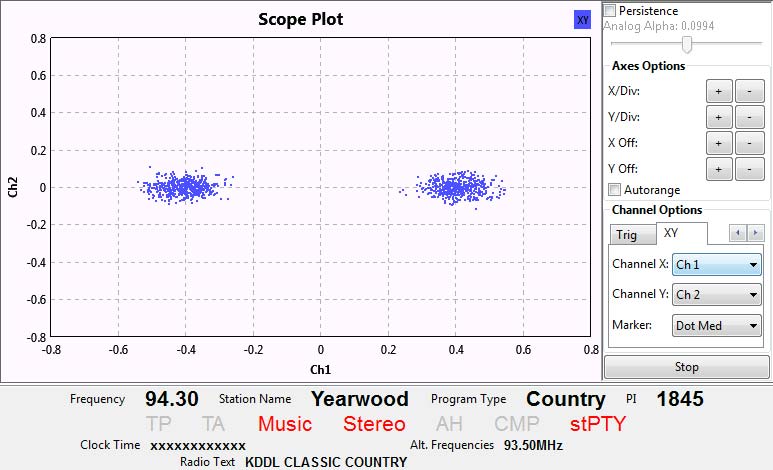
FIGURE 7. Signal constellation displayed by Scope Sink block (top) and decoded RDS program information displayed by RDS Panel block (bottom).

Figure 8 depicts the GRC flowgraph for a FM monophonic receiver that allows reception of SCA subcarrier programming, if the subcarrier is available. As before, the monophonic FM receiver shown in the upper part of the flowgraph is identical to that shown back in Figure 2 and functions in the same way.

FIGURE 8. GRC flowgraph of an FM monophonic receiver that includes SCA reception capability.

This time, the Frequency Xlating FIR Filter block shifts the desired SCA signal to baseband according to the variable channel controlled by the GUI Chooser Block. Selections for several SCA channels as well as RDS are included, so you can “hear” what RDS sounds like if you wish.

The Frequency Xlating FIR Filter block filters the signal according to the parameters listed in the Low-Pass Filter Taps block. Next, the signal is demodulated by the FM Demod block and scaled according to the variable gain_sca by the Multiply Constant block. (The “gain” option in the FM Demod block doesn’t seem to work as it should, so a multiply block is used instead to control volume of the SCA signal.)

Subsidiary Communications Authority (SCA)

According to the FCC, “A subcarrier, known also as Subsidiary Communications Authority or SCA, is a separate audio or data channel that is transmitted along with the main audio signal over a broadcast station. These subcarrier channels are not receivable with a regular radio; special receivers are required. Subcarriers are used for many different purposes, including (but not limited to) paging, inventory distribution, bus dispatching, stock market reports, traffic control signal switching, point-to-point or multipoint messages, foreign language programming, radio reading services ... radio broadcast data systems (RBDS), station control and meter reading, utility load management, and muzak. A broadcast station may transmit more than one subcarrier signal.”

The FCC allocation for SCA dates to the switch of the FM broadcast band from its original 42-50 MHz allocation to the 88-108 MHz allocation in the mid-1940s. The intent of SCA was to provide the nascent FM broadcast industry an additional revenue stream to defray their business and equipment costs.

Unauthorized reception of SCA broadcasts may violate the Communications Act of 1934 which states that “no one may receive, or assist in receiving, any radio communication to which they are not entitled and use that information for their own benefit.” This certainly prohibits any commercial use of the information in these broadcasts.

You should be authorized to receive programming which is non-commercial in nature, such as reading services that are commonly broadcast by NPR affiliated public broadcasting stations. To err on the side of caution, however, you should contact the FM station and request permission authorizing reception of their subcarrier programming for non-commercial, educational, or hobby purposes.

Finally, setting “Num Inputs = 2” in the Audio Sink block enables stereo operation and makes both the monophonic audio and SCA audio signals audible simultaneously with each volume controlled by a GUI Slider block.

Receiving FM stereo is the next stop on our tour of the FM broadcast band. Figure 9 depicts the GRC flowgraph for a basic FM stereophonic receiver that uses the WBFM Receive PLL block. This block accomplishes the tasks necessary to receive FM stereo: Separation and demodulation of the L + R and L - R signals; and then demultiplexing to separate them into the L and R stereo audio channels.

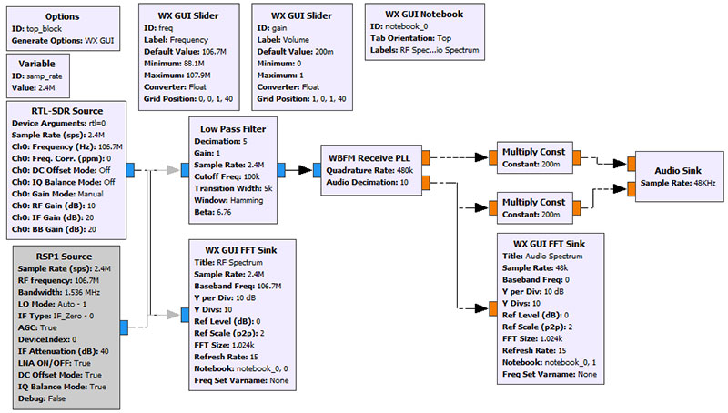
FIGURE 9. GRC flowgraph of a basic FM stereo receiver.

The receiver works beautifully, but it doesn’t provide much insight into its operation since most of the complexity is hidden inside one block.

Figure 10 is a GRC flowgraph that implements FM stereo reception using individual blocks, which allows for greater insight into how stereo reception is accomplished. The L + R signal is obtained in a manner identical to that shown previously in Figure 2, but two additional paths are necessary to recover the L - R signal from the composite baseband signal.

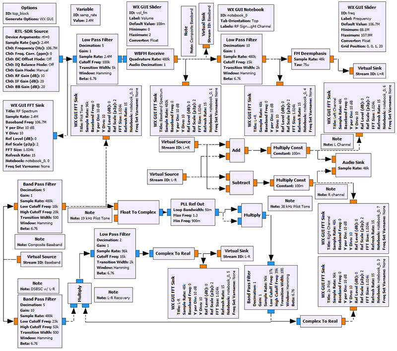
FIGURE 10. GRC flowgraph of a discrete block FM stereo receiver.

The first path uses a bandpass filter to select the 19 kHz pilot tone out of the composite baseband signal; regenerates the tone using a PLL Ref Out block (which implements phased locked loop carrier recovery); doubles the frequency with a Multiply block from 19 kHz to 38 kHz; and then bandpass filters to eliminate everything but the 38 kHz tone.

The second path bandpass filters the composite baseband signal to recover the double sideband suppressed carrier modulation containing the L - R signal; multiplies by the 38 kHz tone to translate it to baseband; and then low pass filters to recover the L - R signal.

The final step is to use Add and Subtract blocks to recover the individual L and R audio channels from the sum and difference of L + R and L - R before sending them to the Audio Sink block to make the sound audible by way of the PC’s speakers. An important advantage of this approach is that it allows us to break out the spectra of the signals along the receive chain as shown in Figure 11.

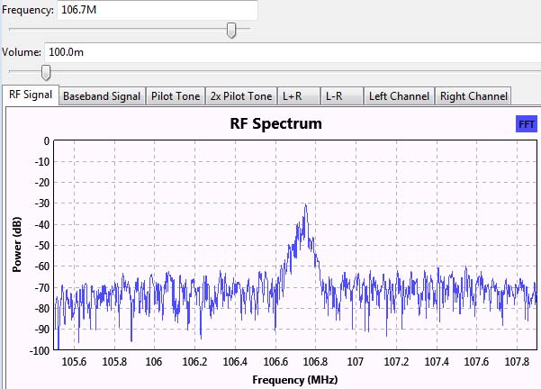
FIGURE 11. Screen capture of FM stereo receiver in operation. Tabs display spectra of signals along the receive chain.

The tabs in this figure permit the user to view FFT plots of the spectra of the following signals: RF signal; composite baseband signal; 19 kHz pilot tone; 38 kHz tone; L + R signal, L - R signal; L audio channel; and R audio channel.

I think the ability to display signals in the time (scope plot) and frequency (FFT plot) domains makes GRC an especially valuable educational tool when it comes to understanding how to put the theory of SDR into practice.

I hope you have as much fun building FM broadcast band receivers using GRC and learning about SDR as I did in preparing this article for you to read. I’m happy to respond to your questions or comments about this article. Please email me at [email protected]. NV